UNIT 4
CHEMICAL BONDING AND MOLECULAR STRUCTURE
Objectives
After studying this Unit, you will be able to
- understand Kössel-Lewis approach to chemical bonding;
- explain the octet rule and its limitations, draw Lewis structures of simple molecules;
- explain the formation of different types of bonds;
- describe the VSEPR theory and predict the geometry of simple molecules;
- explain the valence bond approach for the formation of covalent bonds;
- predict the directional properties of covalent bonds;
- explain the different types of hybridisation involving $s, p$ and $d$ orbitals and draw shapes of simple covalent molecules;
- describe the molecular orbital theory of homonuclear diatomic molecules;
- explain the concept of hydrogen bond.
Researchers are continually identifying novel chemical species, systematically cataloging their characteristics, and endeavoring to elucidate phenomena using current theoretical frameworks. When existing knowledge proves insufficient, they refine established perspectives or develop fresh theoretical constructs to account for recent empirical observations.
Substances are composed of either a single type of element or diverse elemental constituents. Typically, under ambient conditions, no element exists as an isolated atom in nature, with the notable exception of the noble gases. Nonetheless, atomic aggregates frequently co-exist as distinct species, each exhibiting unique properties; these aggregates are termed molecules. It is evident that an inherent force must bind these constituent atoms within molecular structures. This attractive interaction, which unites diverse components (such as atoms or ions) within different chemical entities, is defined as a chemical bond. Given that chemical compounds are formed through the varied association of atoms from different elements, several fundamental inquiries emerge. What impels atoms to combine? Why are specific atomic combinations favored while others are not? What accounts for the distinct geometries observed in molecules? In response to these questions, a range of theories and conceptual frameworks have been progressively developed. These include the Kössel-Lewis approach, the Valence Shell Electron Pair Repulsion (VSEPR) Theory, the Valence Bond (VB) Theory, and the Molecular Orbital (MO) Theory. The progression of valence theories and the elucidation of chemical bond characteristics have been intimately linked with advancements in our comprehension of atomic structure, elemental electronic configurations, and the periodic classification of elements. All systems inherently strive for enhanced stability, and
chemical bonding represents a natural mechanism for reducing a system's energy to achieve this stable state.
4.1 KÖSSEL-LEWIS APPROACH TO CHEMICAL BONDING
Numerous endeavors sought to elucidate chemical bond formation through the lens of electron behavior. However, it was not until 1916 that Kössel and Lewis, working independently, achieved a compelling and comprehensive explanation. Their pioneering efforts yielded the initial coherent theory of valence, fundamentally rooted in the observed chemical inertness of noble gases.
Lewis conceptualized the atom as comprising a positively charged 'Kernel'—encompassing the nucleus and all inner-shell electrons—surrounded by an outer shell capable of holding up to eight electrons. He posited that these eight electrons would occupy the vertices of a cube encircling the 'Kernel'. For instance, a sodium atom's single outer-shell electron would occupy one such vertex, whereas a noble gas atom would have all eight vertices filled. This complete complement of eight electrons, known as an octet, signifies an especially stable electronic configuration.
Lewis advanced the hypothesis that atoms attain this stable octet configuration through the formation of chemical bonds. Illustratively, in the interaction between sodium and chlorine, stability is achieved by the complete transfer of an electron from sodium to chlorine, resulting in the formation of $\mathrm{Na^{+}}$ and $\mathrm{Cl^-}$ ions. Conversely, for entities such as $\mathrm{Cl}_2$ , $\mathrm{H}_2^+$ , and $\mathrm{F}_2^+$ , the linkage is established through the mutual sharing of an electron pair between constituent atoms. In both scenarios, the fundamental outcome is that each involved atom completes a stable outer octet of electrons.
Lewis Symbols: During molecular formation, participation in chemical bonding is restricted exclusively to the outermost shell electrons, which are consequently termed valence electrons. The electrons residing in inner shells are largely shielded and typically do not engage in bonding interactions. The American chemist G.N. Lewis devised a straightforward system of notation to depict the valence electrons within an atom, known as Lewis symbols. For instance, the Lewis symbols corresponding to the elements of the second period are presented below:

Significance of Lewis Symbols: The quantity of dots placed around an element's symbol directly indicates its number of valence electrons. This count of valence electrons is instrumental in determining an element's characteristic, or group, valence. Typically, an element's group valence is ascertained either by directly using the number of dots in its Lewis symbol or by subtracting that number of dots (or valence electrons) from eight.
Kössel, in relation to chemical bonding, drew attention to the following facts:
- He noted that within the periodic classification of elements, the intensely electronegative halogen elements and the highly electropositive alkali metals are situated apart from each other by the intervening noble gases;
- The genesis of a negatively charged ion from a halogen atom and a positively charged ion from an alkali metal atom is intrinsically linked to the acquisition and relinquishment of an electron by these atoms, respectively;
- The resulting negative and positive ions achieve electronic configurations characteristic of stable noble gases. These noble gases, with the singular exception of helium which possesses a duplet of electrons, exhibit an exceptionally stable external shell arrangement comprising eight (octet) electrons, described by the configuration $ns^2 np^6$ .
- The stability of these oppositely charged ions is attributed to the inherent electrostatic forces of attraction between them.
As an illustrative example, the genesis of sodium chloride (NaCl) from its constituent elements, sodium and chlorine, can be elucidated following the aforementioned paradigm:
$ \begin{array}{l} \mathrm {N a} \quad \rightarrow \quad \mathrm {N a} ^ {+} + \mathrm {e} ^ {-} \ [ \mathrm {N e} ] 3 \mathrm {s} ^ {1} \quad [ \mathrm {N e} ] \ \mathrm {C l} + \mathrm {e} ^ {-} \rightarrow \mathrm {C l} ^ {-} \ [ \mathrm {N e} ] 3 s ^ {2} 3 p ^ {5} \quad [ \mathrm {N e} ] 3 s ^ {2} 3 p ^ {6} \text {or} [ \mathrm {A r} ] \ \mathrm {N a} ^ {+} + \mathrm {C l} ^ {-} \rightarrow \mathrm {N a C l} \text {or} \mathrm {N a} ^ {+} \mathrm {C l} ^ {-} \ \end{array} $
In a parallel fashion, the genesis of calcium fluoride ($\mathrm{CaF}_2$) can be delineated as follows:
$ \begin{array}{l} \mathrm {C a} \quad \rightarrow \quad \mathrm {C a} ^ {2 +} + 2 \mathrm {e} ^ {-} \ [ \mathrm {A r} ] 4 s ^ {2} \quad [ \mathrm {A r} ] \ \mathrm {F} + \mathrm {e} ^ {-} \rightarrow \mathrm {F} ^ {-} \ [ \mathrm {H e} ] 2 s ^ {2} 2 p ^ {5} \quad [ \mathrm {H e} ] 2 s ^ {2} 2 p ^ {6} \text {or} [ \mathrm {N e} ] \ \mathrm {C a} ^ {2 +} + 2 \mathrm {F} ^ {-} \rightarrow \mathrm {C a F} _ {2} \text {or} \mathrm {C a} ^ {2 +} (\mathrm {F} ^ {-}) _ {2} \ \end{array} $
The chemical linkage established through the electrostatic attractive forces between these oppositely charged ions was designated as
the electrovalent bond. Consequently, electrovalence corresponds precisely to the magnitude of the unit charge(s) borne by an ion. For instance, calcium is attributed a positive electrovalence of two, whereas chlorine possesses a negative electrovalence of one.
The theoretical propositions advanced by Kössel underpin contemporary understandings concerning the genesis of ions via electron transfer and the subsequent aggregation into ionic crystalline structures. His perspectives have demonstrated substantial utility in facilitating both the comprehension and systematic classification of ionic compounds. Concurrently, he acknowledged that a considerable proportion of chemical compounds deviated from the explanatory framework provided by these principles.
4.1.1 Octet Rule
In 1916, Kössel and Lewis formulated a significant hypothesis regarding the chemical association between atoms, termed the electronic theory of chemical bonding. This theory posits that atoms achieve combination through one of two mechanisms: either by the complete relocation of valence electrons from one atom to another (involving either acquisition or donation), or by the mutual contribution and sharing of valence electrons. The primary objective of these processes is for atoms to attain a stable configuration of eight electrons in their outermost electron shells, a principle commonly referred to as the octet rule.
4.1.2 Covalent Bond
In 1919, Langmuir advanced Lewis's original hypotheses, discarding the concept of a static, cubical arrangement for the octet and concurrently coining the phrase "covalent bond." The principles of the Lewis-Langmuir theory are effectively elucidated by examining the genesis of the chlorine molecule, $\mathrm{Cl}_2$. A singular chlorine atom, possessing the electronic configuration $[\mathrm{Ne}]3s^2 3p^3$, requires one additional electron to achieve the electron arrangement characteristic of argon. The assembly of the $\mathrm{Cl}_2$ molecule is predicated upon the mutual sharing of a pair of electrons between the two constituent chlorine atoms, wherein each chlorine atom furnishes one electron to this shared pair. Through this mechanism, both
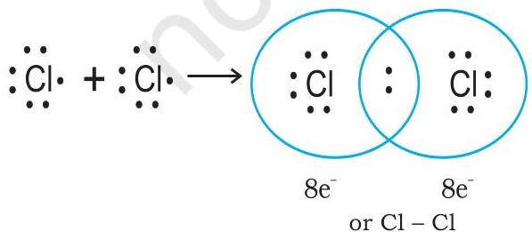 Covalent bond between two Cl atoms
chlorine atoms successfully acquire the stable outer-shell octet characteristic of the closest noble gas, which is argon.
In these representations, individual electrons are symbolized by dots. Configurations of this nature are designated as Lewis dot structures.
Lewis dot structures are also applicable for depicting various other molecules, irrespective of whether their constituent atoms are identical or distinct. The fundamental prerequisites for their formation include:
- Every chemical bond arises from the mutual sharing of an electron pair between participating atoms.
- Each atom involved in the combination donates a minimum of one electron to the shared pair.
- The atoms that combine achieve the electron configurations of noble gases in their outermost shells through the process of electron sharing.
- Consequently, the development of covalent bonds within water and carbon tetrachloride molecules can be illustrated as follows:
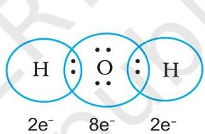 H atoms attain a duplet of electrons and O, the octet
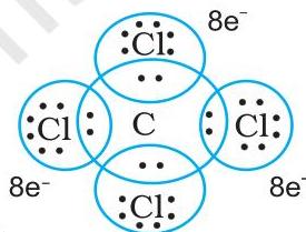 Each of the four Cl atoms along with the C atom attains octet of electrons
Consequently, when two atoms engage in the sharing of a single electron pair, they are described as being connected by a single covalent bond. Numerous compounds, however, feature the presence of multiple bonds between their constituent atoms. The genesis of multiple bonds implies the mutual sharing of more than one electron pair between two atoms. Should two atoms share two distinct pairs of electrons, the resulting covalent linkage between them is termed a double bond. For instance, within the carbon dioxide molecule, $\mathrm{CO}_2$, there exist two double bonds bridging the carbon and oxygen atoms. Analogously, in the ethene molecule, the pair of carbon atoms are interconnected by a double bond.
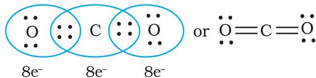 Double bonds in $CO_2$ molecule
The formation of a triple bond occurs when two atoms involved in a chemical combination share three pairs of electrons, exemplified by the two nitrogen atoms in the $\mathbf{N}_2$ molecule and the two carbon atoms within the ethyne molecule.
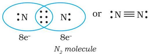
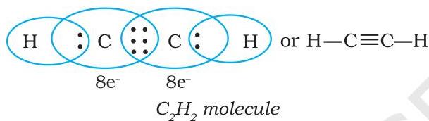
4.1.3 Lewis Representation of Simple Molecules (the Lewis Structures)
Lewis dot structures offer a conceptual representation of chemical bonding in both molecules and ions, focusing on shared electron pairs and adherence to the octet rule. Although this depiction might not comprehensively elucidate a molecule's complete bonding characteristics and behavior, it significantly contributes to grasping its fundamental formation and inherent properties. Consequently, constructing Lewis dot structures for molecules proves to be highly advantageous. The methodology for drawing Lewis dot structures involves the subsequent steps:
- To determine the total electron count necessary for formulating these structures, one sums the valence electrons contributed by all constituent atoms. For instance, in the $\mathrm{CH}_4$ molecule, a total of eight valence electrons are accessible for bonding (four originating from the carbon atom and one from each of the four hydrogen atoms).
- In the case of anions, each unit of negative charge necessitates the incorporation of an additional electron into the total count. Conversely, for cations, each positive charge unit corresponds to the removal of one electron from the overall sum of valence electrons. As an illustration, the $\mathrm{CO}{3}^{2-}$ ion's two negative charges signify the presence of two electrons beyond what the neutral atoms alone would supply. Similarly, for the $\mathrm{NH}{4}^{+}$ ion, a single positive charge denotes the subtraction of one electron from the collective valence electrons of the neutral atomic ensemble.
- Upon identifying the chemical symbols of the constituent atoms and possessing insight into the compound's skeletal arrangement (whether established or deduced through logical inference), the total electron count can be readily allocated as shared bonding pairs among the atoms, commensurate with the aggregate number of bonds.
- Typically, the atom exhibiting the lowest electronegativity assumes the central position within a molecule or ion. For example, in both $\mathrm{NF}3$ and $\mathrm{CO}{3}^{2-}$ , nitrogen and carbon, respectively, serve as the central atoms, while fluorine and oxygen are situated at the peripheral locations.
- Subsequent to assigning shared electron pairs for single bonds, any residual electron pairs are then employed for the formation of multiple bonds or exist as non-bonding lone pairs. The fundamental criterion governing this distribution is that every bonded atom ultimately achieves an octet of electrons.
Lewis representations of a few molecules/ ions are given in Table 4.1.
Table 4.1 The Lewis Representation of Some Molecules
| Molecule/Ion | Lewis Representation | |
|---|---|---|
| H3 | H: H* | H-H |
| O3 | :O::O: | :O=O: |
| O3 | :O:O: | :O*O: |
| NF3 | :F: N:F: | :F-N-F: |
| :F: | :F: | |
| CO3+ | [O:O:O:O-] | [O:O:O-]2- |
| [O:O:O:O-] | [O:O:O-]2- | |
| HNO3 | O:O:O:O: | O=N-O-H |
| O: | O: |
Every hydrogen atom achieves the electron configuration characteristic of helium (a pair of electrons).
CHEMISTRY
Problem 4.1
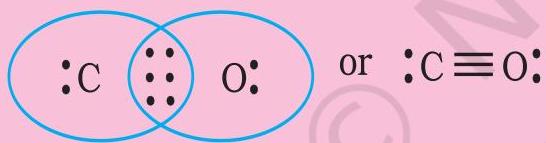
Illustrate the Lewis dot structure for the carbon monoxide (CO) molecule.
Solution
Step 1. Determine the cumulative count of valence electrons contributed by both carbon and oxygen atoms. The electron configurations for the outermost (valence) shells of carbon and oxygen atoms are $2s^2 2p^2$ and $2s^2 2p^4$, respectively. Consequently, the total number of valence electrons accessible for bonding is $4 + 6 = 10$.
Step 2. The foundational skeletal arrangement for the CO molecule is represented as: C O
Step 3. Formulate a single covalent bond (comprising one shared electron pair) between the carbon and oxygen atoms, subsequently fulfilling the octet rule for oxygen. The two remaining electrons are then positioned as a lone pair on the carbon atom.
$ \because \mathrm{C} \equiv \mathrm{O} \equiv \mathrm{O} \quad \text{or} \quad \therefore \mathrm{C} - \mathrm{O} \equiv \mathrm{O} $
Such an arrangement fails to satisfy the octet requirement for carbon, necessitating the formation of multiple bonds (specifically, a triple bond) between the carbon and oxygen atoms. This modification ultimately ensures compliance with the octet rule for both constituent atoms.
Problem 4.2
Write the Lewis structure of the nitrite ion, $\mathrm{NO}_2^-$.
Solution
Step 1. To determine the Lewis structure for the nitrite ion, $\mathrm{NO}_2^-$, the initial step involves calculating the total count of valence electrons from the nitrogen atom, the oxygen atoms, and the single negative charge (which contributes one additional electron).
$ \begin{array}{l} \mathrm{N}(2s^2 2p^4), \mathrm{O}(2s^2 2p^4) \ 5 + (2 \times 6) + 1 = 18 \text{ electrons} \end{array} $
Step 2. Next, establish the fundamental atomic arrangement, positioning the nitrogen atom centrally with the two oxygen atoms bonded to it. The skeletal structure of $\mathrm{NO}_2^-$ is thus: O N O
Step 3. Initially, single covalent bonds (each representing one shared electron pair) are formed between the central nitrogen atom and each peripheral oxygen atom. This typically satisfies the octet rule for the oxygen atoms. However, if the remaining electrons are allocated solely as lone pairs, the nitrogen atom's octet remains incomplete.
$ \boxed{\begin{array}{c c c} \vdots & \text{O} & \text{N} \ \vdots & \ddots & \end{array} \begin{array}{c c c} \vdots & \text{O} \ \vdots & \ddots & \end{array}} $
Consequently, it becomes necessary to introduce multiple bonding, specifically a double bond, between the nitrogen atom and one of the oxygen atoms. This leads to the depiction of resonant Lewis structures.
$ \begin{array}{l} \boxed{\begin{array}{c c c} \mathrm{O} & \mathrm{N} & \mathrm{O} \ \vdots & \ddots & \end{array} } \ \text{or} \ \boxed{\begin{array}{c c c} \mathrm{O} = \mathrm{N} - \mathrm{O} \ \vdots & \ddots & \end{array} } \quad \text{or} \quad \boxed{\begin{array}{c c c} \mathrm{O} - \mathrm{N} = \mathrm{O} \ \vdots & \ddots & \end{array} } \end{array} $
4.1.4 Formal Charge
While Lewis dot structures generally do not depict the precise geometric arrangement of atoms within molecules, it is possible to attribute a conceptual charge, known as formal charge, to individual atoms. For polyatomic ions, the overall charge is distributed across the entire ion, rather than being localized on a single atom. The formal charge for an atom within a polyatomic species (molecule or ion) is precisely defined as the disparity between the count of valence electrons the atom possesses in its isolated, unbonded state and the electron count assigned to that atom within a specific Lewis structural representation. This quantity is calculated using the following formula: $ \begin{aligned} \text{Formal charge (F.C.)} &= \text{Total valence electrons in free atom} \ &\quad - \text{Total non-bonding (lone pair) electrons} \ &\quad - \frac{1}{2} \times \text{Total bonding (shared) electrons}
\end{aligned} $
This method of electron assignment for formal charge calculation assumes that an atom participating in a bond within the molecule is allocated one electron from each shared electron pair, while entirely retaining both electrons from any lone pair it possesses.
To illustrate this concept, let us examine the ozone molecule, $\mathrm{O}_3$. Its Lewis structure can be depicted as shown below:
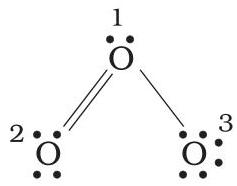
The constituent atoms have been sequentially labeled as 1, 2, and 3. The formal charge determined for each is as follows:
For the central oxygen atom, designated 1:
$ = 6 - 2 - \frac {1}{2} (6) = + 1 $
For the terminal oxygen atom, designated 2:
$ = 6 - 4 - \frac {1}{2} (4) = 0 $
For the terminal oxygen atom, designated 3:
$ = 6 - 6 - \frac {1}{2} (2) = - 1 $
Consequently, the $\mathrm{O}_3$ molecule, incorporating these calculated formal charges, is depicted below:
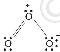
It is crucial to recognize that formal charges do not correspond to the actual distribution of charge or charge separation existing within a molecule. Their primary function, when inscribed on atoms within a Lewis structure, is to facilitate the accounting of valence electrons. Furthermore, formal charges serve as a valuable criterion for discerning the most stable, lowest-energy Lewis structure among several plausible arrangements for a particular chemical species. Typically, the most energetically favorable structure is characterized by the smallest magnitudes of formal charges on its constituent atoms. Fundamentally, the concept of formal charge is predicated on a simplified, purely covalent bonding model where electron pairs are presumed to be shared symmetrically between adjacent atoms.
4.1.5 Limitations of the Octet Rule
While the octet rule proves valuable, it does not hold true in all instances. Its primary utility lies in elucidating the structures of the majority of organic compounds, and its applicability is predominantly observed among elements of the second period in the periodic table. However, the octet rule is subject to three principal categories of exceptions.
The incomplete octet of the central atom
Certain compounds exhibit a phenomenon where the central atom is surrounded by fewer than eight electrons. This characteristic is particularly prevalent in elements possessing fewer than four valence electrons. Illustrative examples include LiCl, $\mathrm{BeH}_2$, and $\mathrm{BCl}_3$.
Li:Cl H:Be:H Cl:B:Cl
Lithium, beryllium, and boron inherently possess only one, two, and three valence electrons, respectively. Additional compounds demonstrating this behavior are $\mathrm{AlCl}_3$ and $\mathrm{BF}_3$.
Odd-electron molecules
For molecules containing an odd total number of electrons, such as nitric oxide (NO) and nitrogen dioxide ($\mathrm{NO}_2$), the octet rule cannot be universally fulfilled for every constituent atom.
$ \stackrel {\leftrightarrow} {\mathrm {N}} = \stackrel {\leftrightarrow} {\mathrm {O}} \quad \stackrel {\leftrightarrow} {\mathrm {O}} = \stackrel {\leftrightarrow} {\mathrm {N}} - \stackrel {\leftrightarrow} {\mathrm {O}}: $
The expanded octet
For elements situated in the third period and subsequent periods of the periodic table, $3d$ orbitals become accessible for chemical bonding, in addition to their $3s$ and $3p$ orbitals. Within various compounds involving these elements, the central atom can accommodate more than eight valence electrons. This phenomenon is referred to as an expanded octet. Evidently, the octet rule is not applicable under these circumstances.
Some of the examples of such compounds are: $\mathrm{PF}_5$, $\mathrm{SF}_6$, $\mathrm{H}_2\mathrm{SO}_4$ and a number of coordination compounds.
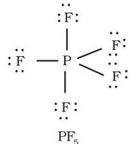 10 electrons around the P atom
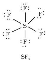 12 electrons around the S atom
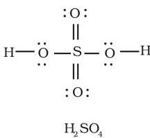 12 electrons around the S atom
It is noteworthy that sulfur can also establish numerous compounds where the octet rule is adhered to. For instance, in sulfur dichloride, the central sulfur atom is surrounded by an octet of electrons.
$ \text{:Cl: — S — :Cl:} \quad \text{or} \quad \text{Cl : S : Cl} $
Other drawbacks of the octet theory
- The octet rule's foundation rests upon the chemical inertness of noble gases. Nevertheless, certain noble gases (such as xenon and krypton) are known to combine with oxygen and fluorine, yielding a variety of compounds like $\mathrm{XeF}_2$, $\mathrm{KrF}_2$, $\mathrm{XeOF}_2$, etc.
- This theoretical framework does not account for the geometric shapes of molecules.
- It fails to provide an explanation for the relative stability of molecules, offering no insight into their energetic properties.
4.2 IONIC OR ELECTROVALENT BOND
Based on the Kössel and Lewis conceptualization of ionic bond formation, it is evident that the genesis of ionic compounds is primarily contingent upon:
- The facility with which positive and negative ions are generated from their respective neutral atoms;
- The spatial arrangement of the positive and negative ions within the solid state, specifically the lattice structure of the crystalline compound.
The formation of a positive ion involves ionization, which is the removal of electron(s) from a neutral atom. Conversely, the creation of a negative ion entails the addition of electron(s) to a neutral atom.
$ \mathrm{M}(\mathrm{g}) \quad \rightarrow \quad \mathrm{M}^{\prime}(\mathrm{g}) + \mathrm{e}^{-}; $
Ionization enthalpy
$ \mathrm{X}(\mathrm{g}) + \mathrm{e}^{-} \rightarrow \mathrm{X}^{-}(\mathrm{g}); $
Electron gain enthalpy
$ \mathrm{M}^{\prime}(\mathrm{g}) + \mathrm{X}^{-}(\mathrm{g}) \rightarrow \mathrm{MX}(\mathrm{s}) $
The electron gain enthalpy, $\Delta_{\mathrm{eq}}H$, represents the enthalpy change (as detailed in Unit 3) that occurs when a gas-phase atom in its ground state acquires an electron. This electron acquisition process can be either exothermic or endothermic. In contrast, ionization is invariably an endothermic process. Electron affinity is defined as the negative value of the energy change accompanying electron gain.
Evidently, ionic bonds are more readily formed between elements possessing comparatively low ionization enthalpies and those exhibiting significantly negative electron gain enthalpy values.
Most ionic compounds feature cations derived from metallic elements and anions originating from non-metallic elements. The ammonium ion, $\mathrm{NH}_4^+$ (composed of two non-metallic elements), stands as an exception, forming the cation in numerous ionic compounds.
Ionic compounds, in their crystalline state, consist of orderly three-dimensional arrangements of cations and anions, held together by strong coulombic interaction energies. These compounds crystallize into various crystal structures, which are determined by factors such as the size of the ions, their packing arrangements, and other considerations. For instance, the crystal structure of sodium chloride, NaCl (commonly known as rock salt), is illustrated below.
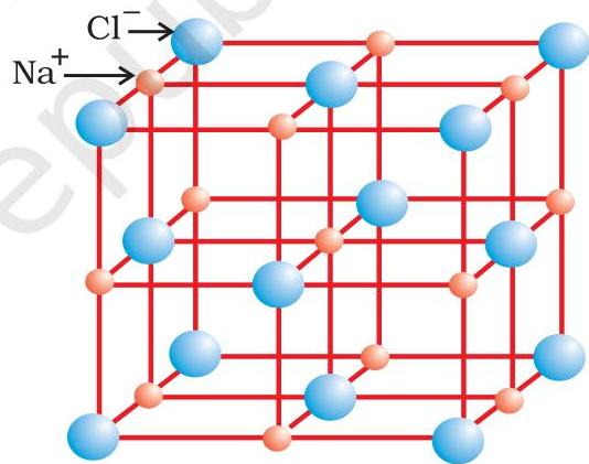 Rock salt structure
In ionic solids, the combined sum of the electron gain enthalpy and the ionization enthalpy may be positive; however, the crystal structure still achieves stability due to the substantial energy released during the formation of the crystal lattice. For example, the ionization enthalpy for the formation of $\mathrm{Na}^{+}(\mathrm{g})$ from $\mathrm{Na}(\mathrm{g})$ is $495.8\ \mathrm{kJ\ mol^{-1}}$, while the electron gain enthalpy for the transformation $\mathrm{Cl}(\mathrm{g}) + \mathrm{e}^{-} \rightarrow \mathrm{Cl}^{-}(\mathrm{g})$ is only $-348.7\ \mathrm{kJ\ mol^{-1}}$. The sum of these two values, $147.1\ \mathrm{kJ\ mol^{-1}}$, is more than compensated for by the highly exothermic enthalpy of lattice formation of $\mathrm{NaCl}(\mathrm{s})$ ($-788\ \mathrm{kJ\ mol^{-1}}$). Therefore, the energy released in the processes is more than the
CHEMICAL BONDING AND MOLECULAR STRUCTURE
energy absorbed. Consequently, the stability of an ionic compound is qualitatively assessed through its lattice enthalpy of formation, rather than solely by the attainment of an electron octet around the constituent ions in their gaseous state.
Given the pivotal role of lattice enthalpy in the genesis of ionic compounds, a more comprehensive exploration of this concept is warranted.
4.2.1 Lattice Enthalpy
Lattice Enthalpy for an ionic solid is formally characterized as the energy input necessary to fully dissociate one mole of the solid ionic substance into its gaseous ionic components. Illustratively, the lattice enthalpy for sodium chloride (NaCl) is $788\mathrm{kJ mol^{-1}}$. This value signifies that an energy expenditure of 788 kJ is requisite to dissociate one mole of solid NaCl into one mole of gaseous $\mathrm{Na^{+}}$ ions and one mole of gaseous $\mathrm{Cl^-}$ ions, achieving an infinite separation between them.
This phenomenon encompasses both the electrostatic attractive forces operating between oppositely charged ions and the repulsive forces acting between similarly charged ions. Given the inherent three-dimensional structure of a solid crystal, a direct computation of lattice enthalpy solely based on these attractive and repulsive interactions is not feasible. Consequently, parameters pertaining to the crystal's geometric arrangement must also be incorporated into such calculations.
4.3 BOND PARAMETERS
4.3.1 Bond Length
The bond length refers to the equilibrium separation between the nuclei of two atoms that are chemically bonded within a molecular structure. The determination of bond lengths is achieved through advanced techniques such as spectroscopy, X-ray diffraction, and electron diffraction, topics which are explored in greater detail in advanced academic curricula. Each constituent atom within a bonded pair contributes to the overall bond length, as illustrated in Fig. 4.1. Specifically, for a covalent bond, this individual atomic contribution is designated as the covalent radius.
The covalent radius is approximately quantified as the effective radius of an atom's core when it is in direct contact with the core of a neighboring atom within a chemical bond. For two identical atoms linked by a covalent bond within the same molecule, the covalent radius is precisely half of the internuclear distance between them.
Fig. 4.1 The bond length in a covalent molecule $AB$ .
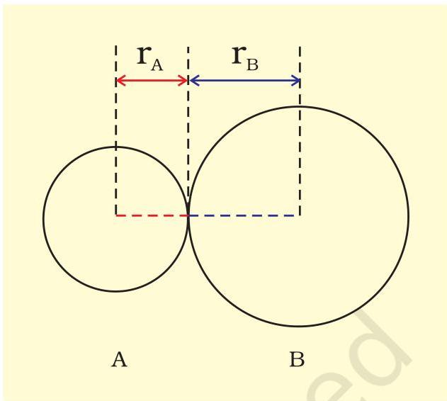 $R = r_{A} + r_{B}$ (where $R$ signifies the bond length, and $r_A$ and $r_B$ denote the covalent radii of atoms A and B, respectively)
The van der Waals radius, in contrast, characterizes the overall spatial extent of an atom, encompassing its valence shell, when it is not engaged in chemical bonding. Moreover, for two identical atoms situated in distinct molecules within a solid state, the van der Waals radius is determined as half of the internuclear separation between them. Figure 4.2 illustrates the covalent and van der Waals radii specific to a chlorine molecule.
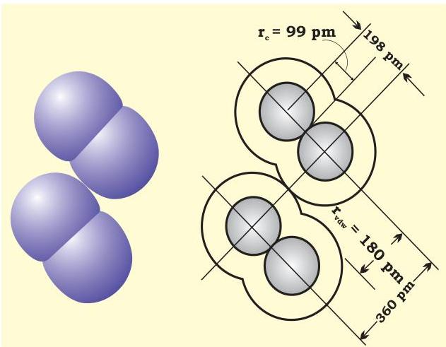 Fig. 4.2 Covalent and van der Waals radii in a chlorine molecule. The inner circles correspond to the size of the chlorine atom ( $r_{chlor}$ and $r_{c}$ are van der Waals and covalent radii respectively).
Table 4.2 presents characteristic average bond lengths for single, double, and triple bonds. Bond lengths for various common molecules are provided in Table 4.3. The covalent radii for several common elements are enumerated in Table 4.4.
4.3.2 Bond Angle
The bond angle refers to the angular separation between the orbitals housing bonding electron pairs surrounding the central atom within a molecule or a complex ion. This value is quantified in degrees and can be empirically ascertained through spectroscopic techniques. It offers insights into the spatial arrangement of orbitals around the central atom in a given species, thereby aiding in the elucidation of its molecular geometry. For instance, the H–O–H bond angle in a water molecule is depicted below:
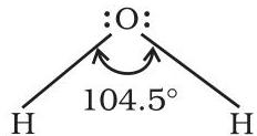
4.3.3 Bond Enthalpy
Bond enthalpy is characterized as the energy input necessary to dissociate one mole of a specific bond type connecting two atoms in their gaseous phase. Its standard unit is kilojoules per mole (kJ mol⁻¹). To illustrate, the H–H bond enthalpy within a hydrogen molecule measures 435.8 kJ mol⁻¹.
$ \mathrm{H}2(\mathrm{g}) \rightarrow \mathrm{H}(\mathrm{g}) + \mathrm{H}(\mathrm{g}); \Delta{\mathrm{e}} H^{\circ} = 435.8 , \mathrm{kJ} , \mathrm{mol}^{-1} $
Analogously, the bond enthalpy values for molecules featuring multiple bonds, such as O₂ and N₂, are presented as follows:
$ \begin{array}{l} \mathrm{O}2(\mathrm{O} = \mathrm{O})(\mathrm{g}) \rightarrow \mathrm{O}(\mathrm{g}) + \mathrm{O}(\mathrm{g}); \ \Delta{\mathrm{e}} H^{\circ} = 498 , \mathrm{kJ} , \mathrm{mol}^{-1} \ \end{array} $
$ \begin{array}{l} \mathrm{N}2(\mathrm{N} \equiv \mathrm{N})(\mathrm{g}) \rightarrow \mathrm{N}(\mathrm{g}) + \mathrm{N}(\mathrm{g}); \ \Delta{\mathrm{e}} H^{\circ} = 946.0 , \mathrm{kJ} , \mathrm{mol}^{-1} \ \end{array} $
A crucial implication is that a greater bond dissociation enthalpy correlates directly with a stronger chemical bond within the molecule. Considering heteronuclear diatomic molecules, such as hydrogen chloride (HCl), we observe:
$ \mathrm{HCl}(\mathrm{g}) \rightarrow \mathrm{H}(\mathrm{g}) + \mathrm{Cl}(\mathrm{g}); \Delta_{\mathrm{e}} H^{\circ} = 431.0 , \mathrm{kJ} , \mathrm{mol}^{-1} $
For polyatomic molecules, assessing bond strength presents a greater degree of complexity. For instance, in the water (H₂O) molecule, the energy required to cleave each of the two O–H bonds differs.
Table 4.2 Average Bond Lengths for Some Single, Double and Triple Bonds
| Bond Type | Covalent Bond Length (pm) |
|---|---|
| O–H | 96 |
| C–H | 107 |
| N–O | 136 |
| C–O | 143 |
| C–N | 143 |
| C–C | 154 |
| C=O | 121 |
| N=O | 122 |
| C=C | 133 |
| C=N | 138 |
| C≡N | 116 |
| C≡C | 120 |
Table 4.3 Bond Lengths in Some Common Molecules
| Molecule | Bond Length (pm) |
|---|---|
| H₂ (H–H) | 74 |
| F₂ (F–F) | 144 |
| Cl₂ (Cl–Cl) | 199 |
| Br₂ (Br–Br) | 228 |
| I₂ (I–I) | 267 |
| N₂ (N≡N) | 109 |
| O₂ (O=O) | 121 |
| HF (H–F) | 92 |
| HCl (H–Cl) | 127 |
| HBr (H–Br) | 141 |
| HI (H–I) | 160 |
Table 4.4 Covalent Radii, *r_cov/(pm)
| H | 37 | ||||||
|---|---|---|---|---|---|---|---|
| C | 77(1) | N | 74 (1) | O | 66(1) | F | 64 |
| 67 (2) | 65(2) | 57 (2) | Cl | 99 | |||
| 60(3) | 55(3) | ||||||
| P | 110 | S | 104(1) | Br | 114 | ||
| 95(2) | |||||||
| As | 121 | Se | 104 | I | 133 | ||
| Sb | 141 | Te | 137 |
* The values cited are for single bonds, except where otherwise indicated in parenthesis. (See also Unit 3 for periodic trends).
CHEMICAL BONDING AND MOLECULAR STRUCTURE
$ \begin{array}{l} \mathrm {H} _ {2} \mathrm {O} (\mathrm {g}) \rightarrow \mathrm {H} (\mathrm {g}) + \mathrm {O H} (\mathrm {g}); \Delta_ {\mathrm {g}} H _ {1} ^ {\ominus} = 5 0 2 \mathrm {k J m o l} ^ {- 1} \ \mathrm {O H} (\mathrm {g}) \rightarrow \mathrm {H} (\mathrm {g}) + \mathrm {O} (\mathrm {g}); \Delta_ {\mathrm {g}} H _ {2} ^ {\ominus} = 4 2 7 \mathrm {k J m o l} ^ {- 1} \ \end{array} $
The discrepancy in the $\Delta_{\mathrm{g}}H^{\ominus}$ values indicates a modification in the properties of the second O-H bond, attributable to its altered chemical environment. Consequently, the energy required to cleave an O-H bond can vary across different molecular contexts, such as in $\mathrm{C}_2\mathrm{H}_5\mathrm{OH}$ (ethanol) compared to water. Thus, for molecules comprising multiple atoms, the concept of mean or average bond enthalpy is employed. This value is calculated by dividing the aggregate bond dissociation enthalpy by the total count of bonds severed, as demonstrated subsequently for the water molecule.
$ \begin{array}{l} \text {Average bond enthalpy} = \frac {5 0 2 + 4 2 7}{2} \ = 4 6 4. 5 \mathrm {k J m o l} ^ {- 1} \ \end{array} $
4.3.4 Bond Order
Within the Lewis framework for describing covalent bonds, the Bond Order quantifies the number of shared bonds existing between two atoms within a molecule. For instance, in $\mathrm{H}{2}$ (characterized by one shared electron pair), in $\mathrm{O}{3}$ (possessing two shared electron pairs), and in $\mathrm{N}{2}$ (featuring three shared electron pairs), the respective bond orders are 1, 2, and 3. Similarly, for carbon monoxide (CO), where carbon and oxygen share three electron pairs, the bond order is 3. Notably, $\mathrm{N}{2}$ exhibits a bond order of 3, and its associated $\Delta_{8}H^{\ominus}$ is $946\mathrm{kJ mol^{-1}}$, placing it among the highest values for diatomic molecules.
Molecules and ions that are isoelectronic exhibit identical bond orders. For example, $\mathbf{F}_3$ and $\mathrm{O}_4^{2-}$ share a bond order of 1, while $\mathbf{N}_3$, CO, and $\mathrm{NO}^+$ all have a bond order of 3.
A significant correlation, instrumental in comprehending molecular stabilities, indicates that an escalation in bond order corresponds to an increase in bond enthalpy and a reduction in bond length.
4.3.5 Resonance Structures
It is frequently observed that a singular Lewis structure proves insufficient to accurately represent a molecule's characteristics in alignment with its experimentally determined parameters. As an illustration, the ozone molecule, $\mathrm{O}_3$, can be depicted equivalently by structures I and II, as presented below:
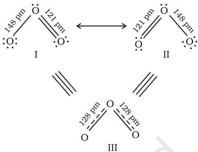 Fig. 4.3 Resonance in the $O_3$ molecule
(structures I and II represent the two canonical forms while the structure III is the resonance hybrid)
In both of these structural representations, one finds a single O-O bond and a $\mathrm{O = O}$ double bond. The typical bond lengths for an O-O single bond and a $\mathrm{O = O}$ double bond are $148\mathrm{pm}$ and $121\mathrm{pm}$, respectively. However, experimental measurements reveal that the oxygen-oxygen bond lengths within the $\mathrm{O_3}$ molecule are identical, measuring $128~\mathrm{pm}$. Consequently, the oxygen-oxygen bonds in $\mathrm{O_3}$ possess characteristics intermediate between those of a double and a single bond. Evidently, neither of the two Lewis structures presented above can adequately convey this observed reality.
The principle of resonance was introduced to address the challenges encountered in accurately illustrating the structures of molecules such as $\mathrm{O}_3$. According to the resonance concept, whenever a single Lewis structure fails to precisely describe a molecule, multiple structures—each possessing similar energy, identical nuclear positions, and comparable distributions of bonding and non-bonding electron pairs—are considered as canonical structures. These canonical structures collectively contribute to a hybrid representation that more accurately depicts the molecule. Thus, for $\mathrm{O}_3$, the two structures previously illustrated serve as the canonical or resonance structures, and their hybrid, denoted as structure III, offers a more accurate representation of the $\mathrm{O_3}$ molecule. This composite representation is also termed a resonance hybrid. Resonance phenomena are conventionally indicated by a double-headed arrow.
Further instances of resonance structures include the carbonate ion and the carbon dioxide molecule.
Problem 4.3
Explain the structure of $\mathrm{CO}_{3}^{2-}$ ion in terms of resonance.
Solution
A solitary Lewis structure, predicated on the existence of two single bonds and one double bond between carbon and oxygen atoms, proves insufficient for an accurate depiction of the molecule because it suggests disparate bond characteristics. However, experimental observations conclusively indicate that all carbon-oxygen bonds within the $\mathrm{CO}_{3}^{2-}$ ion exhibit equivalence. Consequently, the most appropriate representation for the carbonate ion is as a resonance hybrid, formed by the superposition of the canonical forms designated as I, II, and III, as illustrated below.
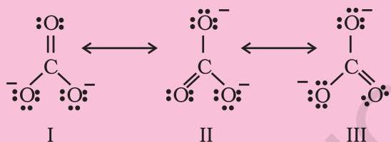 Fig. 4.4 Resonance in $\mathrm{CO}_{3}^{2-}$, I, II and III represent the three canonical forms.
Problem 4.4
Explain the structure of $\mathrm{CO}_{2}$ molecule.
Solution
The carbon-oxygen bond length in the $\mathrm{CO}{2}$ molecule, as determined through experimental methods, measures $115\mathrm{pm}$. For comparison, the typical bond lengths for a carbon-oxygen double bond $(\mathrm{C} = \mathrm{O})$ and a carbon-oxygen triple bond $(\mathrm{C} \equiv \mathrm{O})$ are $121\mathrm{pm}$ and $110~\mathrm{pm}$, respectively. It is evident that the carbon-oxygen bond length observed in $\mathrm{CO}{2}$ ($115~\mathrm{pm}$) lies between the values characteristic of a $\mathrm{C} = \mathrm{O}$ bond and a $\mathrm{C} \equiv \mathrm{O}$ bond. Clearly, a singular Lewis structure cannot accurately portray this intermediate bonding scenario. Therefore, it becomes essential to construct multiple Lewis structures and to conceptualize the structure of $\mathrm{CO}_{2}$ as a hybrid comprising the canonical, or resonance, forms I, II, and III.
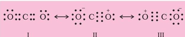 Fig. 4.5 Resonance in $\mathrm{CO}_{2}$ molecule, I, II and III represent the three canonical forms.
In general, it may be stated that
- Resonance confers stability upon the molecule, as the energy of the resonance hybrid is inherently lower than that of any single hypothetical canonical structure; and,
- Resonance results in the averaging of bond characteristics across the entire molecular entity.
Consequently, the energy associated with the $\mathrm{O}_2$ resonance hybrid is lower than that of either of its two canonical forms, I and II (Fig. 4.3).
Numerous misunderstandings are frequently associated with the concept of resonance, and these require clarification. It is important to recall that:
- The canonical forms possess no actual physical existence.
- The molecule does not transition or exist for varying durations in one canonical form and then others.
- No equilibrium, analogous to that observed between tautomeric forms (e.g., keto and enol) in tautomerism, exists between canonical forms.
- The molecule itself possesses a singular structure, which is the resonance hybrid of its canonical forms, and this singular structure cannot be accurately represented by any individual Lewis structure.
4.3.6 Polarity of Bonds
The conceptualization of a bond as exclusively 100% ionic or covalent serves as an idealized model. In actuality, no chemical bond or compound exhibits a purely covalent or ionic nature. Even within a covalent bond formed between two hydrogen atoms, a minute degree of ionic character is inherently present.
When a covalent bond arises from the interaction of two identical atoms, such as in $\mathrm{H}{2}$, $\mathrm{O}{2}$, $\mathrm{Cl}{2}$, $\mathrm{N}{2}$, or $\mathrm{F}_{2}$, the shared
electron pair experiences equivalent attractive forces from both nuclei. As a result, the electron pair resides precisely midway between the two equivalent atomic centers, forming what is termed a nonpolar covalent bond. Conversely, within a heteronuclear molecule like HF, the electron pair shared between the two constituent atoms is unequally distributed, exhibiting a greater displacement towards the fluorine atom. This phenomenon occurs because fluorine possesses a significantly higher electronegativity (as discussed in Unit 3) compared to hydrogen. The resulting covalent linkage is thus classified as a polar covalent bond.
This polarization leads to the development of a dipole moment within the molecule, an attribute defined as the product of the magnitude of the separated charge and the spatial separation between the centroids of positive and negative charge. This quantity is conventionally symbolized by the Greek letter $\mu$. Its mathematical representation is as follows:
Dipole moment $(\mu) = \text{charge (Q)} \times \text{distance of separation (r)}$
The dipole moment is typically quantified in Debye (D) units. The relevant conversion factor is provided as:
$ 1 \mathrm {D} = 3. 3 3 5 6 4 \times 1 0 ^ {- 3 0} \mathrm {C m} $
where $C$ is coulomb and $m$ is meter.
Furthermore, dipole moment is inherently a vector quantity. By established convention, it is visually represented by a small arrow whose tail originates from the negative charge center and whose head points towards the positive charge center. However, in chemical notation, the existence of a dipole moment is commonly indicated on a molecule's Lewis structure using a crossed arrow $(+\rightarrow)$. In this representation, the cross signifies the positive terminus, and the arrowhead designates the negative terminus. For instance, the dipole moment of hydrogen fluoride (HF) can be illustrated as:

The depicted arrow signifies the displacement of electron density within the molecular structure. It is important to observe that the orientation of this crossed arrow runs counter to the standard representation of the dipole moment vector.
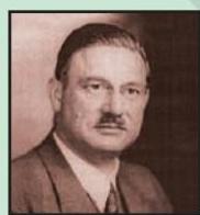
In 1936, the Dutch chemist Peter Debye was awarded the Nobel Prize for his contributions to the fields of X-ray diffraction and dipole moments. In recognition of his achievements, the magnitude of the dipole moment is conventionally expressed in Debye units.
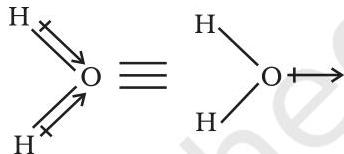
For polyatomic molecules, the overall dipole moment is contingent not solely on the individual dipole moments of their constituent bonds, termed bond dipoles, but also significantly on the three-dimensional spatial configuration of these bonds within the molecule. Consequently, the molecular dipole moment is determined as the vector sum of the dipole moments contributed by its various bonds. As an illustration, consider the $\mathrm{H}_2\mathrm{O}$ molecule, which possesses a bent geometry. Here, the two O-H bonds are spatially oriented at an angle of $104.5^{\circ}$. The net dipole moment, measured at $6.17 \times 10^{-30} \mathrm{Cm}$ (where $1\mathrm{D} = 3.33564 \times 10^{-30} \mathrm{Cm}$), represents the vector resultant of the individual dipole moments from these two O-H bonds.
 (a) Bond dipole
(b) Resultant dipole moment
(a) Bond dipole
(b) Resultant dipole moment
Net Dipole moment, $\mu = 1.85\mathrm{D}$
$ = 1. 8 5 \times 3. 3 3 5 6 4 \times 1 0 ^ {- 3 0} \mathrm {C m} = 6. 1 7 \times 1 0 ^ {- 3 0} \mathrm {C m} $
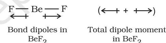
The $\mathrm{BeF}_2$ molecule exhibits a zero dipole moment. This phenomenon occurs because its two bond dipoles, being of equivalent magnitude, are oriented in diametrically opposing directions, thereby mutually nullifying their respective effects.
Even in a tetra-atomic molecule such as $\mathrm{BF}_3$, the dipole moment registers as zero. This outcome arises despite the B-F bonds being positioned at $120^{\circ}$ angles relative to each other, because the collective contribution of the three bond moments results in a net sum of zero, specifically due to the resultant of any two bond moments being equal in magnitude and opposite in direction to the third.
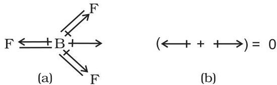
$BF_{3}$ molecule; representation of (a) bond dipoles and (b) total dipole moment
Consider an intriguing comparison between the $\mathrm{NH}_3$ and $\mathrm{NF}_3$ molecules. Both species adopt a pyramidal geometry, each featuring a lone pair of electrons situated on the central nitrogen atom. Despite fluorine possessing greater electronegativity than nitrogen, the resultant
dipole moment of $\mathrm{NH}_3$ ($4.90 \times 10^{-30} \mathrm{Cm}$) significantly exceeds that of $\mathrm{NF}_3$ ($0.8 \times 10^{-30} \mathrm{Cm}$). This discrepancy is attributable to the orientation of the orbital dipole arising from the lone pair: in $\mathrm{NH}_3$, this orbital dipole aligns with the direction of the resultant dipole moment from the $\mathrm{N}-\mathrm{H}$ bonds, thereby augmenting it. Conversely, in $\mathrm{NF}_3$, the orbital dipole is oriented in opposition to the resultant dipole moment of the three N-F bonds. This opposing orbital dipole from the lone pair consequently diminishes the overall effect of the resultant $\mathrm{N}-\mathrm{F}$ bond moments, leading to the comparatively low dipole moment observed in $\mathrm{NF}_3$, as illustrated subsequently:
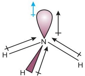 Resultant dipole moment in $\mathrm{NH}_3 = 4.90\times 10^{-30}\mathrm{Cm}$
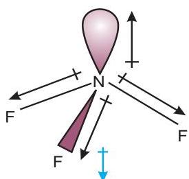 Resultant dipole moment in $\mathrm{NF}_3 = 0.80\times 10^{-30}\mathrm{Cm}$
Dipole moments of some molecules are shown in Table 4.5.
While all covalent bonds possess a degree of ionic character, ionic bonds similarly exhibit a partial covalent nature. Fajans elucidated the factors influencing this partial covalent character in ionic compounds through the subsequent principles:
- The covalent character of an ionic bond increases with a diminished cationic radius and an expanded anionic radius.
- A higher charge on the cation directly correlates with a more pronounced covalent character in the ionic bond.
- Among cations of equivalent size and charge, those possessing an electronic configuration of $(n - 1)d^{n}ns^{n}$ (characteristic of transition metals) demonstrate greater polarizing power than those with a noble gas configuration, $ns^2 np^6$ (typical of alkali and alkaline earth metal cations).
The cation exerts a polarizing effect on the anion, drawing the electron cloud towards itself. This process elevates the electron density within the internuclear region, a phenomenon analogous to the formation of a covalent bond, which is characterized by the accumulation of electron charge between the nuclei. The extent of covalent character within an ionic bond is consequently determined by three primary factors: the polarizing capability of the cation, the polarizability of the anion, and the resulting degree of distortion (polarization) undergone by the anion.
4.4 THE VALENCE SHELL ELECTRON PAIR REPULSION (VSEPR) THEORY
As previously established, the Lewis concept proves insufficient for elucidating the precise geometries of molecules. The VSEPR theory, conversely, furnishes a straightforward methodology for forecasting the shapes of covalent compounds. Sidgwick
Table 4.5 Dipole Moments of Selected Molecules
| Type of Molecule | Example | Dipole Moment, (\mu) (D) | Geometry |
|---|---|---|---|
| Molecule (AB) | HF | 1.78 | linear |
| HCl | 1.07 | linear | |
| HBr | 0.79 | linear | |
| HI | 0.38 | linear | |
| (H_2) | 0 | linear | |
| Molecule ((AB_2)) | (H_2O) | 1.85 | bent |
| (H_2S) | 0.95 | bent | |
| (CO_2) | 0 | linear | |
| Molecule ((AB_3)) | (NH_3) | 1.47 | trigonal-pyramidal |
| (NF_3) | 0.23 | trigonal-pyramidal | |
| (BF_3) | 0 | trigonal-planar | |
| Molecule ((AB_4)) | (CH_4) | 0 | tetrahedral |
| (CHCl_3) | 1.04 | tetrahedral | |
| (CCl_4) | 0 | tetrahedral |
and Powell, in 1940, originally put forth a foundational theory rooted in the repulsive interactions among electron pairs within the valence shell of atoms. This theoretical framework subsequently underwent significant development and redefinition by Nyholm and Gillespie in 1957.
The fundamental tenets of VSEPR theory are as follows:
- The ultimate geometry of a molecule is contingent upon the aggregate number of valence shell electron pairs (whether bonding or non-bonding) surrounding its central atom.
- Within the valence shell, electron pairs exhibit mutual repulsion due to the inherent negative charge of their electron clouds.
- Consequently, these electron pairs tend to orient themselves in spatial configurations that minimize repulsive forces, thereby maximizing the distances separating them.
- The valence shell is conceptually treated as a spherical entity, with the electron pairs localizing on its surface to achieve the greatest possible separation from one another.
- A multiple bond is construed as functionally equivalent to a single electron pair, meaning the two or three electron pairs comprising a multiple bond are regarded as a singular 'super pair'.
- In instances where a molecule can be represented by two or more resonance structures, the VSEPR model remains applicable to each individual resonance form.
The hierarchy of repulsive forces among electron pairs is observed to diminish in the following sequence:
Lone pair (lp) - Lone pair (lp) > Lone pair (lp) - Bond pair (bp) > Bond pair (bp) - Bond pair (bp)
Nyholm and Gillespie (1957) further refined the VSEPR model by elucidating the crucial difference between non-bonding (lone) and bonding electron pairs. While lone pairs are exclusively localized on the central atom, each bonding pair is shared between two atomic centers. As a direct consequence, the electron density associated with lone pairs in a molecule occupies a greater spatial volume compared to that of bonding pairs. This increased spatial occupancy of lone pairs engenders stronger repulsive interactions between lone pairs themselves, relative to the repulsions between a lone pair and a bond pair, and between two bond pairs. Such differential repulsive effects invariably lead to divergences from idealized molecular geometries and modifications in observed bond angles within molecules.
For the purpose of predicting the geometric forms of molecules using VSEPR theory, it is practical to classify molecules into two principal categories: (i) those where the central atom lacks any lone pairs, and (ii) those where the central atom possesses one or more lone pairs.
Table 4.6 illustrates the spatial arrangement of electron pairs around a central atom A (devoid of lone pairs) and the resultant geometries for various molecules/ions of the AB type. Table 4.7 presents the forms of several simple molecules and ions where the central atom contains one or more lone pairs. Table 4.8 elucidates the underlying causes for geometrical distortions observed in molecules.
As exemplified in Table 4.6, for compounds designated as $\mathrm{AB}_2$, $\mathrm{AB}_3$, $\mathrm{AB}_4$, $\mathrm{AB}_5$, and $\mathrm{AB}_6$, the spatial configuration of electron pairs and the attendant B atoms surrounding the central atom A are characterized as linear, trigonal planar, tetrahedral, trigonal-bipyramidal, and octahedral, respectively. This type of arrangement is observable in molecules such as $\mathrm{BF}_3$ ($\mathrm{AB}_3$), $\mathrm{CH}_4$ ($\mathrm{AB}_4$), and $\mathrm{PCl}_5$ ($\mathrm{AB}_5$), as represented by their ball-and-stick models below.
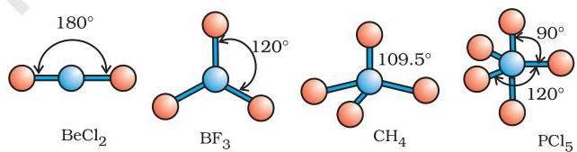 Fig. 4.6 The shapes of molecules in which central atom has no lone pair
The VSEPR (Valence Shell Electron Pair Repulsion) theory offers a reliable method for forecasting the geometries of numerous molecules, particularly those involving $p$-block elements, with considerable precision. Its utility extends to accurately ascertaining molecular configurations even when the energetic distinctions among potential structures are minimal. However, the foundational theoretical principles of VSEPR concerning how electron pair repulsions influence molecular shapes remain ambiguous and are an ongoing subject of academic debate.
CHEMISTRY
Table 4.6 Geometry of Molecules in which the Central Atom has No Lone Pair of Electrons
| Number of electron pairs | Arrangement of electron pairs | Molecular geometry | Examples |
|---|---|---|---|
| 2 | B—A—B Linear | BeCl_{2}, HgCl_{2} |
|
| 3 | B A B Trigonal planar | BF_{3} |
|
| 4 | B B B Tetrahedral | CH_{4}, NH_{4}^{+} |
|
| 5 | B B B Trigonal bipyramidal | PCl_{5} |
|
| 6 | B B B Octahedral | SF_{6} |
CHEMICAL BONDING AND MOLECULAR STRUCTURE
CHEMISTRY
Table 4.8 Shapes of Molecules containing Bond Pair and Lone Pair
| Molecule type | No. of bonding pairs | No. of lone pairs | Arrangement of electrons | Shape | Reason for the shape acquired |
|---|---|---|---|---|---|
| (AB_2E) | 2 | 1 | Trigonal planar | Bent | Although theoretically expected to exhibit a trigonal planar configuration, this molecular type adopts a bent or V-shaped geometry. This deviation arises because the repulsion between lone pairs and bond pairs significantly exceeds that between bond pairs, leading to a reduction in the bond angle from (120^\circ) to (119.5^\circ). |
| (AB_3E) | 3 | 1 | Tetrahedral | Trigonal pyramidal | If a bond pair occupied the position of the lone pair, the molecule would possess a tetrahedral shape. However, the presence of a single lone pair results in a trigonal pyramidal structure. This is attributed to the greater repulsion between lone pairs and bond pairs compared to bond pair-bond pair repulsion, causing the bond angle to decrease from (109.5^\circ) to (107^\circ). |
| (AB_2E_2) | 2 | 2 | Tetrahedral | Bent | Were all electron pairs bond pairs, a tetrahedral geometry would be expected. However, with two lone pairs present, the molecule adopts a distorted tetrahedral or angular form. This outcome stems from the hierarchy of repulsions: lone pair-lone pair repulsion is greater than lone pair-bond pair repulsion, which in turn surpasses bond pair-bond pair repulsion. Consequently, the bond angle is diminished from (109.5^\circ) to (104.5^\circ). |
| (AB_4E) | 4 | 1 | Trigonal bipyramidal | See-saw | When the lone pair occupies an axial position, three lone pair-bond pair repulsions occur at (90^\circ). Conversely, if the lone pair is situated in an equatorial position, only two such repulsions exist. Therefore, the equatorial arrangement exhibits greater stability. The resulting molecular configuration is characterized as a distorted tetrahedron, a folded square, or a see-saw shape. |
| (AB_3E_2) | 3 | 2 | Trigonal bipyramidal | T-shape | In the most stable configuration, the lone pairs occupy equatorial positions, leading to fewer lone pair-bond pair repulsions compared with arrangements where lone pairs occupy axial positions. Consequently, the molecule adopts a T-shaped geometry. |
4.5 VALENCE BOND THEORY
While the Lewis approach facilitates the depiction of molecular structures, it proves inadequate in elucidating the fundamental process of chemical bond formation. Furthermore, it offers no rationale for the disparities observed in bond dissociation enthalpies and bond lengths, as exemplified by molecules such as $\mathrm{H}{2}$ (435.8 kJ mol$^{-1}$, 74 pm) and $\mathrm{F}{2}$ (155 kJ mol$^{-1}$, 144 pm), despite both involving the formation of a single covalent bond through electron pair sharing between constituent atoms. The theory also provides no insight into the geometries of polyatomic molecules.
Likewise, the VSEPR theory describes the geometries of uncomplicated molecules, yet it lacks a theoretical explanation for these arrangements and possesses inherent limitations in its applicability. To address these deficiencies, two significant theories grounded in quantum mechanical principles have been developed: valence bond (VB) theory and molecular orbital (MO) theory.
The Valence bond theory was initially proposed by Heitler and London in 1927, subsequently undergoing further development by Pauling and other researchers. An understanding of valence bond theory necessitates familiarity with atomic orbitals, the electronic configurations of elements (as covered in Units 2), the criteria governing the overlap of atomic orbitals, the concept of atomic orbital hybridization, and the principles of variation and superposition. A comprehensive and rigorous examination of VB theory, encompassing these detailed aspects, falls outside the purview of this textbook. Consequently, for pedagogical clarity, the valence bond theory is presented here solely through a qualitative and non-mathematical lens. To commence, we will analyze the formation of the hydrogen molecule, recognized as the most elementary of all molecular species.
Envision two hydrogen atoms, designated A and B, drawing near to one another. Each possesses a nucleus, denoted as $\mathrm{N}{\mathrm{A}}$ and $\mathrm{N}{\mathrm{B}}$ respectively, and their corresponding electrons are represented by $\mathrm{e}{\mathrm{A}}$ and $\mathrm{e}{\mathrm{B}}$. When these two atoms are situated at a considerable separation, no significant interaction exists between them. However, as their proximity increases, novel attractive and repulsive forces commence their operation.
The attractive forces manifest between:
(i) the nucleus of an atom and its own electron, specifically $\mathrm{N}{\mathrm{A}} - \mathrm{e}{\mathrm{A}}$ and $\mathrm{N}{\mathrm{B}} - \mathrm{e}{\mathrm{B}}$.
(ii) the nucleus of one atom and an electron belonging to the other atom, for instance, $\mathrm{N}{\mathrm{A}} - \mathrm{e}{\mathrm{B}}$ and $\mathrm{N}{\mathrm{B}} - \mathrm{e}{\mathrm{A}}$.
Analogously, repulsive interactions manifest between:
(i) the electron clouds of distinct atoms, such as $\mathrm{e_A - e_B}$ (ii) the nuclei of separate atoms, exemplified by $\mathrm{N_A - N_B}$
While attractive forces facilitate the close proximity of two atoms, repulsive forces, conversely, drive them apart (refer to Fig. 4.7).
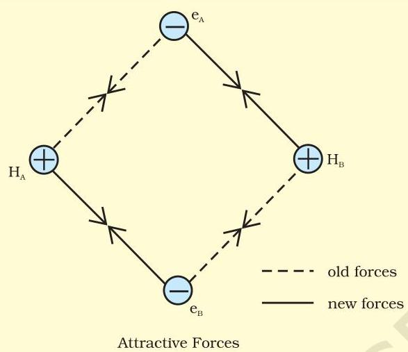
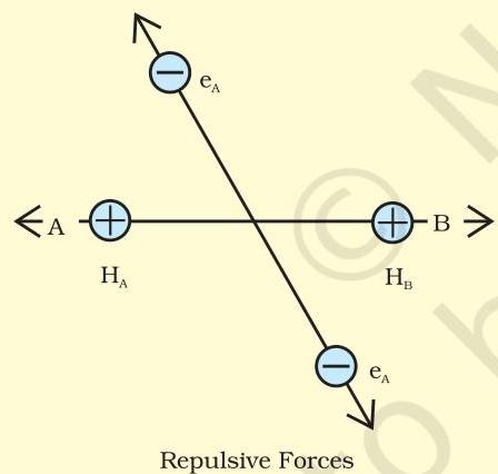 Fig. 4.7 Forces of attraction and repulsion during the formation of $H_{2}$ molecule
Empirical observations indicate that the strength of the emergent attractive forces surpasses that of the emergent repulsive forces. Consequently, as the two atoms draw nearer, their potential energy diminishes. This process culminates in a state where the resultant attractive force is precisely counterbalanced by the repulsive force, leading the system to attain its lowest energy configuration. At this specific point, two hydrogen atoms are considered to be chemically bound, forming a stable molecule characterized by an internuclear separation of $74~\mathrm{pm}$.
Given that energy is liberated during the formation of a chemical bond between two hydrogen atoms, the resultant hydrogen molecule exhibits greater stability compared to its constituent isolated hydrogen atoms. This liberated energy is termed bond enthalpy, and it corresponds to the minimum point on the potential energy curve illustrated in Fig. 4.8. Conversely, a quantity of $435.8\mathrm{kJ}$ of energy must be supplied to cleave one mole of $\mathrm{H}_{2}$ molecules.
$ \mathrm {H} _ {2} (\mathrm {g}) + 4 3 5. 8 \mathrm {k J} \mathrm {m o l} ^ {- 1} \rightarrow \mathrm {H} (\mathrm {g}) + \mathrm {H} (\mathrm {g}) $
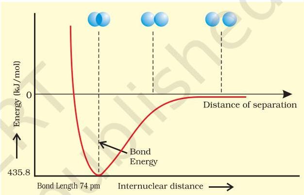 Fig. 4.8 The potential energy curve for the formation of $H_{2}$ molecule as a function of internuclear distance of the $H$ atoms. The minimum in the curve corresponds to the most stable state of $H_{2}$ .
4.5.1 Orbital Overlap Concept
When two hydrogen atoms approach sufficiently close, a state of minimum energy is achieved where their respective atomic orbitals partially interpenetrate. This phenomenon of partial orbital fusion is termed the overlapping of atomic orbitals, leading to the pairing of electrons. The degree to which these orbitals overlap is directly correlated with the strength of the resultant covalent bond. Generally, an increased extent of overlap corresponds to a stronger bond between the two atoms. Consequently, the orbital overlap concept posits that the generation of a covalent bond between two atoms is contingent upon the pairing of valence electrons possessing opposing spins.
4.5.2 Directional Properties of Bonds
As previously established, covalent bonds arise from the overlapping of atomic orbitals. For instance, the hydrogen molecule results from the overlap between the 1s-orbitals of two hydrogen atoms.
For more complex polyatomic molecules, such as $\mathrm{CH}_4$, $\mathrm{NH}_3$, and $\mathrm{H}_2\mathrm{O}$, molecular geometry holds significant importance alongside bond formation. Considerations arise, for example, regarding why the $\mathrm{CH}_4$ molecule exhibits a tetrahedral configuration with HCH bond angles of $109.5^\circ$, or why the $\mathrm{NH}_3$ molecule adopts a pyramidal shape.
The valence bond theory offers an explanation for the geometry, formation, and directional characteristics of bonds in polyatomic species like $\mathrm{CH}_4$, $\mathrm{NH}_3$, and $\mathrm{H}_2\mathrm{O}$, among others, by invoking the principles of orbital overlap and hybridisation.
4.5.3 Overlapping of Atomic Orbitals
When the orbitals of two atoms draw near to facilitate bond formation, their interaction can lead to an overlap that is either positive, negative, or zero. This outcome is determined by the sign (phase) and the spatial orientation of the orbital wave function's amplitude (Fig. 4.9). It is crucial to understand that the positive and negative indicators on the boundary surface diagrams in Fig. 4.9 denote the phase of the orbital wave function and bear no relation to electrical charge. For orbitals to form a bond, they must exhibit the same sign (phase) and spatial orientation; this condition is termed positive overlap. Figure 4.9 illustrates various instances of overlap involving $s$ and $p$ orbitals.
The principle of overlap, serving as the primary determinant for the formation of covalent bonds, applies consistently to both homonuclear and heteronuclear diatomic molecules, as well as to polyatomic compounds. We are aware that molecules such as $\mathrm{CH}_4$, $\mathrm{NH}_3$, and $\mathrm{H}_2\mathrm{O}$ possess tetrahedral, pyramidal, and bent geometries, respectively. It is therefore insightful to employ Valence Bond (VB) theory to ascertain whether these specific molecular shapes can be rationalized through the concept of orbital overlaps.
Let us commence by examining the $\mathrm{CH}_4$ (methane) molecule. The electronic configuration of carbon in its ground state is represented as $[\mathrm{He}]2s^2 2p^2$. In an excited state, this configuration transitions to $[\mathrm{He}]2s^1 2p_x^1 2p_y^1 2p_z^1$. The energetic input required for this excitation is counterbalanced by the energy released as a result of the overlap between the orbitals of carbon and the
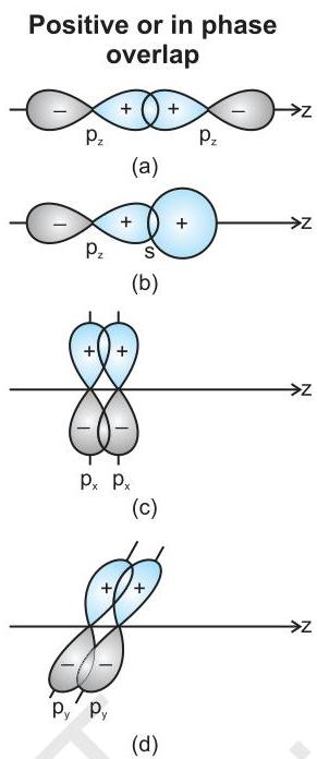
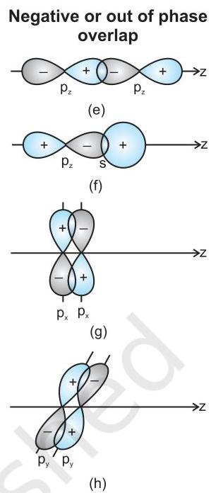
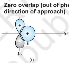 Fig.4.9 Positive, negative and zero overlaps of $s$ and $p$ atomic orbitals
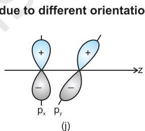
hydrogen atoms. The four atomic orbitals of carbon, each containing an unpaired electron, are capable of overlapping with the $1s$ orbitals of the four hydrogen atoms, which are also singly occupied. This interaction leads to the formation of four C-H bonds. Nevertheless, it will be observed that while the three $p$ orbitals of carbon are oriented at $90^{\circ}$ relative to one another, the HCH angle for these would similarly be $90^{\circ}$. This implies that three of the C-H bonds would be spatially arranged at $90^{\circ}$ to each other. Furthermore, the $2s$ orbital of carbon and the $1s$ orbital of hydrogen are spherically symmetrical, allowing for overlap in any direction. Consequently, the precise orientation of the fourth C-H bond cannot be definitively determined through this simple model. This description fails to align with the experimentally established tetrahedral HCH angles of $109.5^{\circ}$. Evidently, it follows that a straightforward application of atomic orbital overlap principles does not adequately account for the directional characteristics of bonds in $\mathrm{CH}_4$. Employing a similar methodology and line of reasoning, it can be demonstrated that in the case of $\mathrm{NH}_3$ and $\mathrm{H}_2\mathrm{O}$ molecules, the HNH
whereas HOH angles are predicted to be 90°. This theoretical expectation diverges from the experimentally determined bond angles of 107° for NH₃ and 104.5° for H₂O molecules, respectively.
4.5.4 Types of Overlapping and Nature of Covalent Bonds
Covalent bonds can be categorized into two principal forms based on the specific manner in which atomic orbitals interact:
(i) Sigma(σ) bond, and (ii) pi(π) bond
(i) Sigma(σ) bond: This variety of covalent bond arises from the direct, head-to-head (or end-on) alignment and overlap of bonding orbitals along the primary internuclear axis. This interaction is alternatively termed axial overlap. Its formation can occur through any of the subsequent combinations involving atomic orbitals:
- s-s overlapping: This scenario involves the linear overlap of two half-filled s-orbitals precisely along the internuclear axis, as depicted below:

- s-p overlapping: This mode of overlap manifests between a half-filled s-orbital from one atom and a half-filled p-orbital originating from another atom.

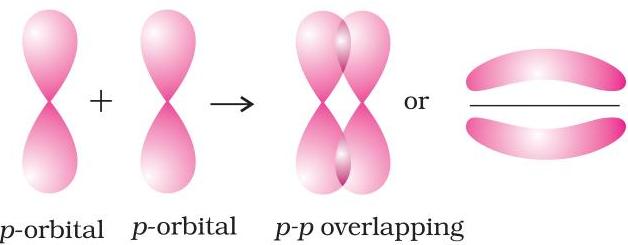
- p-p overlapping: This interaction occurs when half-filled p-orbitals from two distinct, approaching atoms engage in a direct overlap.

(ii) pi(π) bond: The formation of a π bond involves the sidewise overlap of atomic orbitals, where their axes maintain a parallel orientation relative to each other and are simultaneously perpendicular to the internuclear axis. The resultant molecular orbitals from this lateral interaction typically present as two electron density regions, resembling saucer-shaped clouds, situated both above and below the plane defined by the participating atoms.
4.5.5 Strength of Sigma and pi Bonds
The efficacy of a chemical bond is principally governed by the degree of orbital overlap. Sigma bonds are distinguished by a more extensive overlap of atomic orbitals, which confers upon them greater strength compared to pi bonds, where the orbital overlap is considerably less pronounced. Moreover, in the construction of multiple bonds between two atoms in a molecule, it is essential to understand that pi bonds are invariably formed as supplementary components to a primary sigma bond.
4.6 HYBRIDISATION
To elucidate the distinct geometric configurations of polyatomic species such as CH₄, NH₃, and H₂O, Pauling advanced the theory of hybridisation. His proposition posits that atomic orbitals coalesce to generate a novel collection of equivalent orbitals, termed hybrid orbitals. These hybrid orbitals, unlike their pure counterparts, actively participate in bond formation. Hybridisation itself is defined as the procedure involving the commingling of orbitals possessing marginally disparate energy levels, leading to a redistribution of their energies and the subsequent generation of a new ensemble of orbitals characterized by identical energies and spatial forms. For instance, the hybridization of one 2s orbital and three 2p orbitals in a carbon atom results in the genesis of four sp³ hybrid orbitals.
Salient features of hybridisation: The principal characteristics of hybridisation are as follows:
The quantity of hybrid orbitals generated precisely corresponds to the count of atomic orbitals undergoing hybridization.
Hybridized orbitals consistently exhibit equivalence in both their energy levels and spatial configurations.
Hybrid orbitals demonstrate superior efficacy in establishing robust chemical bonds compared to their unhybridized atomic orbital counterparts.
These hybrid orbitals orient themselves in specific spatial directions, a configuration optimized to minimize electron pair repulsion, thereby achieving a stable molecular arrangement. Consequently, the specific mode of hybridisation serves as an indicator of the molecule's overall geometry.
Important conditions for hybridisation
(i) Hybridization exclusively involves orbitals located within the valence shell of an atom. (ii) The orbitals participating in the hybridization process must possess energies that are nearly equivalent. (iii) It is not a prerequisite for electrons to be promoted to higher energy levels prior to hybridization. (iv) Participation in hybridization is not restricted solely to half-filled orbitals; under certain circumstances, fully occupied valence shell orbitals can also engage in this process.
4.6.1 Types of Hybridisation
Hybridization encompasses several classifications, which involve the combination of $s$, $p$, and $d$ atomic orbitals. The distinct categories of hybridization are detailed below:
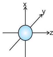
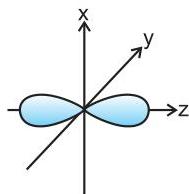
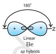
(I) $sp$ hybridisation: This form of hybridization is characterized by the combination of a single $s$ orbital and a single $p$ orbital, leading to the generation of two identical $sp$ hybrid orbitals. For the resulting hybrid orbitals to align themselves along the $z$-axis, the appropriate atomic orbitals for $sp$ hybridization are the $s$ and $p_s$ orbitals. Each resultant $sp$ hybrid orbital exhibits an equal proportion of $s$-character and $p$-character, specifically $50%$ for each. A molecule featuring a central atom that is $sp$-hybridized and directly bonded to two other atoms will adopt a linear molecular geometry. This specific form of hybridization is additionally referred to as diagonal hybridization.
The two $sp$ hybrid orbitals are oriented diametrically opposite to each other along the $z$-axis. They feature prominent positive lobes and significantly smaller negative lobes, a configuration that facilitates enhanced orbital overlap and, consequently, the formation of more robust chemical bonds.
Example of molecule having sp hybridisation
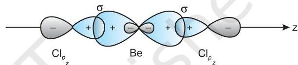
For $\mathbf{BeCl}_2$, the beryllium atom initially possesses a ground state electronic configuration of $1s^2 2s^2$. To achieve its bivalent nature, one of the electrons from the $2s$ orbital is promoted to an unoccupied $2p$ orbital in the excited state. Subsequently, one $2s$ orbital and one $2p$ orbital undergo hybridization, resulting in the formation of two $sp$ hybrid orbitals. These two $sp$ hybrid orbitals adopt an opposing orientation, establishing an angle of $180^{\circ}$ between them. Each of these $sp$ hybrid orbitals then undergoes axial overlap with a $2p$ orbital from a chlorine atom, leading to the formation of two Be-Cl sigma bonds. This process is visually represented in Fig. 4.10.
 (a)
(a)
 (b)
$\mathrm{BeCl}_2$ molecule
Fig.4.10 (a) Formation of sp hybrids from s and p orbitals; (b) Formation of the linear $\mathrm{BeCl}_2$ molecule
(b)
$\mathrm{BeCl}_2$ molecule
Fig.4.10 (a) Formation of sp hybrids from s and p orbitals; (b) Formation of the linear $\mathrm{BeCl}_2$ molecule
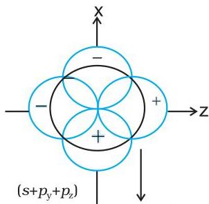
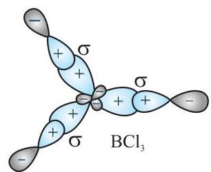
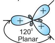
(II) $sp^2$ hybridisation: This form of hybridization involves the combination of one $s$ orbital and two $p$ orbitals to generate three equivalent $sp^2$ hybrid orbitals. Consider the $\mathrm{BCl}_3$ molecule as an illustration. The central boron atom in its ground state exhibits an electronic configuration of $1s^2 2s^2 2p^1$. Upon excitation, one of the $2s$ electrons is promoted to a vacant $2p$ orbital, which consequently provides
boron with three unpaired electrons. These three orbitals—one $2s$ and two $2p$—then undergo hybridization to produce three $sp^2$ hybrid orbitals. The resulting three hybrid orbitals are arranged in a trigonal planar configuration and participate in overlap with the $2p$ orbitals of chlorine atoms, thereby forming three B-Cl bonds. As a result, the $\mathrm{BCl}_3$ molecule (as depicted in Fig. 4.11) exhibits a trigonal planar geometry with a ClBCl bond angle of $120^\circ$.
 $sp^2$ hybrids
Fig.4.11 Formation of $sp^2$ hybrids and the $BCl_3$ molecule
$sp^2$ hybrids
Fig.4.11 Formation of $sp^2$ hybrids and the $BCl_3$ molecule
(III) $sp^3$ hybridisation: This category of hybridization can be elucidated through the example of the $\mathrm{CH}_4$ molecule. It involves the intermixing of one $s$-orbital and three $p$-orbitals from the valence shell to generate four $sp^3$ hybrid orbitals, each possessing equivalent energies and identical shapes. Each $sp^3$ hybrid orbital exhibits a $25%$ $s$-character and a $75%$ $p$-character. These four $sp^3$ hybrid orbitals are spatially directed towards the four vertices of a tetrahedron. The angular separation between any two $sp^3$ hybrid orbitals is $109.5^\circ$, as illustrated in Fig. 4.12.
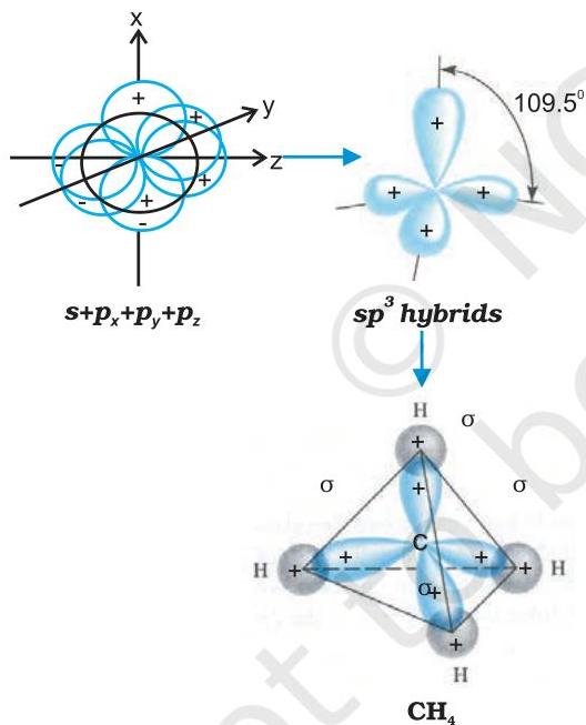 Fig.4.12 Formation of $sp^3$ hybrids by the combination of $s, p_x, p_y$ and $p_x$ atomic orbitals of carbon and the formation of $CH_4$ molecule
The molecular configurations of both $\mathrm{NH}3$ and $\mathrm{H}2\mathrm{O}$ can be elucidated through the concept of $sp^3$ hybridisation. Considering $\mathrm{NH}3$, nitrogen's valence shell electron arrangement in its ground state is characterized by $2\mathrm{S}^{2}2p{x}^{1}2p{y}^{1}2p{z}^{1}$. This leads to the formation of four $sp^3$ hybrid orbitals, three of which contain single, unpaired electrons, while the fourth accommodates a lone pair. The three hybrid orbitals possessing unpaired electrons then engage in an overlap with the 1s orbitals of hydrogen atoms, culminating in the formation of three N-H sigma bonds. It is established that the repulsive force exerted by a lone pair on a bond pair surpasses that between two bond pairs. Consequently, the molecule experiences a distortion, causing the bond angle to decrease from the ideal $109.5^\circ$ to $107^\circ$. The resulting spatial arrangement of this molecule is thus pyramidal, as depicted in Fig. 4.13.
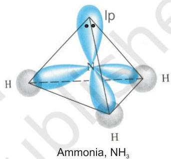 Fig.4.13 Formation of $\mathrm{NH}_3$ molecule
For the $\mathrm{H}_2\mathrm{O}$ molecule, the oxygen atom's four orbitals (comprising one 2s and three 2p orbitals) also participate in $sp^3$ hybridisation. This process generates four $sp^3$ hybrid orbitals; two of these are singly occupied with one electron each, while the remaining two accommodate lone pairs of electrons. These four $sp^3$ hybrid orbitals initially adopt a tetrahedral arrangement. Within this configuration, two vertices are occupied by hydrogen atoms forming bonds, whereas the other two vertices are occupied by the lone pairs. Due to the influence of these lone pairs, the bond angle experiences a contraction, decreasing from the ideal $109.5^\circ$ to $104.5^\circ$ (Fig. 4.14). Consequently, the molecule assumes a V-shape, also known as an angular geometry.
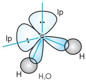 Fig.4.14 Formation of $\mathrm{H}_2\mathrm{O}$ molecule
4.6.2 Other Examples of $sp^3$ , $sp^2$ and $sp$ Hybridisation
$sp^3$ Hybridisation in $C_2H_6$ molecule: Within the ethane molecule, both carbon atoms adopt an $sp^3$ hybridized configuration. An axial overlap occurs between one $sp^3$ hybrid orbital from each carbon atom, establishing a sigma bond between the two carbon centers. The remaining three $sp^3$ hybrid orbitals on each carbon atom are then utilized to form sigma bonds with hydrogen atoms via axial overlap with their respective $s$ orbitals, as detailed in section 4.6.1(iii). Consequently, the carbon-carbon bond in ethane exhibits a length of 154 pm, while each carbon-hydrogen bond measures 109 pm.
$sp^2$ Hybridisation in $C_2H_4$: During the synthesis of the ethene molecule, one $sp^2$ hybrid orbital from a carbon atom engages in axial overlap with an $sp^2$ hybridized orbital from the second carbon atom, resulting in the establishment of a carbon-carbon sigma bond. The two other $sp^2$ hybrid orbitals on each carbon atom are employed to create $sp^2 - s$ sigma bonds with two hydrogen atoms. Concurrently, an unhybridized orbital (specifically, $2p_x$ or $2p_y$) from one carbon atom undergoes lateral overlap with a corresponding orbital from the other carbon atom, leading to the formation of a weaker $\pi$ bond. This $\pi$ bond is characterized by two symmetrical electron clouds positioned above and below the plane defined by the carbon and hydrogen atoms.
Therefore, within the ethene molecule, the carbon-carbon linkage comprises a single $sp^2 - sp^2$ sigma bond and one pi $(\pi)$ bond, which arises from the overlap of $p$ orbitals that did not participate in hybridization and lie perpendicular to the molecular plane; this bond measures 134 pm in length. Each C-H bond is an $sp^2 - s$ sigma bond, with a length of 108 pm. The H-C-H bond angle is observed to be $117.6^\circ$, while the H-C-C angle is $121^\circ$. Figure 4.15 illustrates the formation of both sigma and pi bonds in ethene.
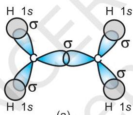 (a)
(a)
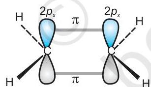 (b)
(b)
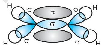 (c)
(c)
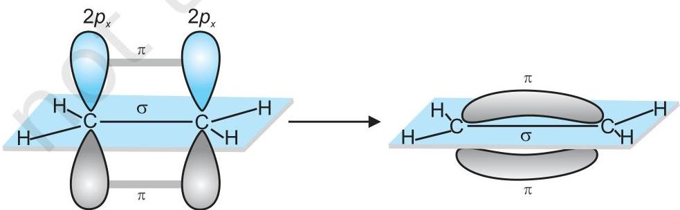 (d)
Fig. 4.15 Formation of sigma and pi bonds in ethene
(d)
Fig. 4.15 Formation of sigma and pi bonds in ethene
$sp$ Hybridisation in $C_2H_2$: In the formation of the ethyne molecule, both carbon atoms undergo $sp$-hybridization, possessing two unhybridized orbitals, specifically $2p_y$ and $2p_x$.
An $sp$ hybrid orbital from one carbon atom engages in axial overlap with an $sp$ hybrid orbital from the other carbon atom, establishing a C–C sigma bond. Simultaneously, the remaining $sp$ hybridized orbital on each carbon atom overlaps axially with the half-filled $s$ orbital of a hydrogen atom, thereby forming sigma ($\sigma$) bonds. Furthermore, each of the two unhybridized $p$ orbitals from both carbon atoms undergoes lateral overlap, resulting in the creation of two $\pi$ bonds between the carbon atoms. Consequently, the triple bond connecting the two carbon atoms is composed of one sigma bond and two pi bonds, as depicted in Fig. 4.16.
4.6.3 Hybridisation of Elements involving d Orbitals
Third-period elements possess d orbitals in addition to their s and p orbitals. The energy levels of the 3d orbitals are comparable to those of the 3s and 3p orbitals. Furthermore, the 3d orbitals also exhibit energies similar to the 4s and 4p orbitals. Consequently, hybridization schemes can involve combinations such as 3s, 3p, and 3d, or alternatively, 3d, 4s, and 4p. However, due to a substantial energy disparity between the 3p and 4s orbitals, hybridization involving 3p, 3d, and 4s orbitals simultaneously is not energetically feasible.
The principal hybridization patterns incorporating s, p, and d orbitals are presented below:
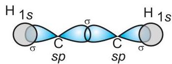 (a)
(a)
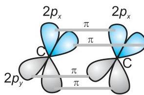 (b)
(b)
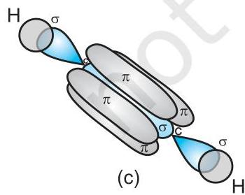 Fig.4.16 Formation of sigma and pi bonds in ethyne
| Shape of molecules/ions | Hybridisation type | Atomic orbitals | Examples |
|---|---|---|---|
| Square planar | $dsp^2$ | $d+s+p(2)$ | $[\mathrm{Ni(CN)_4}]^{2-}$, $[\mathrm{Pt(Cl)_4}]^{2-}$ |
| Trigonal bipyramidal | $sp^2d$ | $s+p(3)+d$ | $\mathrm{PF}_5$, $\mathrm{PCl}_5$ |
| Square pyramidal | $sp^2d^2$ | $s+p(3)+d(2)$ | $\mathrm{BrF}_5$ |
| Octahedral | $sp^2d^2$ | $s+p(3)+d(2)$ | $\mathrm{SF}_6$, $[\mathrm{CrF}_6]^{3-}$ $[\mathrm{Co(NH_3)_6}]^{3+}$ |
| $d^2sp^3$ | $d(2)+s+p(3)$ |
(i) Formation of $PCl_{5}$ ($sp^3d$ hybridisation): The ground state and the excited state outer electronic configurations of phosphorus $(Z=15)$ are represented below.
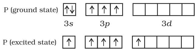
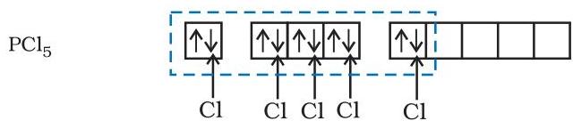 $sp^3d$ hybrid orbitals filled by electron pairs donated by five Cl atoms.
Consequently, a total of five orbitals—specifically, one $s$, three $p$, and one $d$ orbital—become available for hybridization. This process generates a set of five $sp^3 d$ hybrid orbitals, which are geometrically oriented towards the five vertices of a trigonal bipyramidal arrangement, as illustrated in Fig. 4.17.
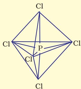 Fig. 4.17 Trigonal bipyramidal geometry of $PCl_{5}$ molecule
It is important to recognize that the bond angles within a trigonal bipyramidal geometry are not all equivalent. In the $\mathrm{PCl}_5$ molecule, the five $sp^3 d$ hybrid orbitals belonging to phosphorus undergo overlap with the singly occupied $p$ orbitals of five chlorine atoms, resulting in the formation of five P-Cl sigma bonds. Three of these P-Cl bonds reside within a single plane, forming angles of $120^\circ$ with each other; these are designated as equatorial bonds. The remaining two P-Cl bonds, positioned one above and one below the equatorial plane, form $90^\circ$ angles with this plane and are known as axial bonds. Due to increased repulsive interactions experienced by the axial bond pairs from the equatorial bond pairs, the axial bonds are observed to be marginally longer and consequently somewhat weaker than their equatorial counterparts. This structural characteristic contributes to the enhanced reactivity of the $\mathrm{PCl}_5$ molecule.
(ii) Formation of $SF_{6}$ ($sp^{3}d^{2}$ hybridisation): For $SF_{6}$, the sulfur atom, positioned centrally, exhibits an outer electronic configuration of $3s^{2}3p^{4}$ in its ground state. Upon excitation, six orbitals become available—specifically, one $s$, three $p$, and two $d$ orbitals—each housing a single electron. These orbitals undergo hybridization, resulting in the formation of six equivalent $sp^{3}d^{2}$ hybrid orbitals. These hybrid orbitals are oriented spatially towards the six vertices of a regular octahedron within the $SF_{6}$ structure. Subsequently, each of these six $sp^3 d^2$ hybrid orbitals engages in an overlap with a singly occupied orbital from a fluorine atom, thereby establishing six S-F sigma bonds. Consequently, the $\mathrm{SF}_6$ molecule adopts a distinct regular octahedral geometry, as depicted in Fig. 4.18.
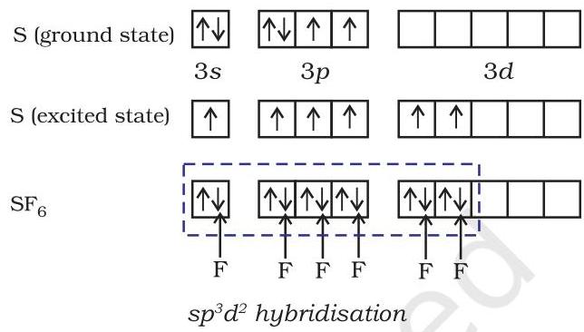
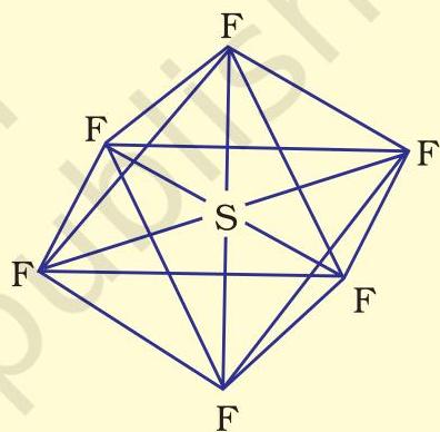 Fig. 4.18 Octahedral geometry of $SF_{6}$ molecule
4.7 MOLECULAR ORBITAL THEORY
The molecular orbital (MO) theory was formulated by F. Hund and R.S. Mulliken in 1932. Its principal characteristics include the following:
(i) Within a molecule, electrons reside in distinct molecular orbitals, much like electrons within individual atoms occupy their respective atomic orbitals. (ii) Atomic orbitals possessing similar energy levels and appropriate symmetry characteristics coalesce to generate molecular orbitals. (iii) An electron situated in an atomic orbital experiences the influence of a single nucleus, whereas an electron within a molecular orbital is affected by two or more nuclei, the precise number being contingent on the atom count in the molecule. Hence,
an atomic orbital is characterized as monocentric, while a molecular orbital is deemed polycentric.
(iv) The quantity of molecular orbitals generated corresponds precisely to the number of atomic orbitals that participate in the combination. For instance, when two atomic orbitals interact, two molecular orbitals emerge: one designated as a bonding molecular orbital and the other termed an antibonding molecular orbital. (v) A bonding molecular orbital possesses a lower energy state, consequently exhibiting enhanced stability compared to its counterpart, the antibonding molecular orbital. (vi) Analogous to how an atomic orbital describes the electron probability distribution surrounding a nucleus in an atom, a molecular orbital delineates the electron probability distribution around an assembly of nuclei within a molecule. (vii) Similar to atomic orbitals, molecular orbitals are populated with electrons following the aufbau principle, while also adhering to Pauli's exclusion principle and Hund's rule.
4.7.1 Formation of Molecular Orbitals Linear Combination of Atomic Orbitals (LCAO)
Within the framework of wave mechanics, atomic orbitals are conceptualized through wave functions, denoted as $(\psi
YoLearn.AI is India's #1 AI tutoring platform for Class 1 to 12, JEE, and NEET preparation.
Students talk to expert AI tutors in real time through live voice calls, solve doubts instantly
on an interactive sketch board, and practice with mock tests, flashcards, quizzes, and slide decks.
Learn from top educators including DC Pandey and other verified teachers who create AI avatars of themselves.
Unlike text-only chatbots, YoLearn.AI lets you speak naturally to your AI tutor — just like a real
one-on-one session. Get step-by-step explanations for Physics, Chemistry, Maths, and Biology
for board exams, JEE Main, JEE Advanced, and NEET.
Prepare for JEE 2026, NEET 2026, and CBSE board exams with personalized mock tests, AI-generated
quizzes, and flashcard makers. Build daily study habits with an AI study buddy designed for Indian students.
Whether you need a Class 10 CBSE tutor, Class 12 board exam help, or full JEE and NEET coaching online,
YoLearn.AI adapts to your grade, syllabus, and learning pace. Start free today on web, iOS, and Android.
Personal 1:1 AI Tutor for CBSE, JEE & NEET Students
Live voice tutoring and doubt solving
Mock tests, flashcards, and exam prep
For school, JEE, and NEET
To illustrate this methodology, we can consider the