Chapter Seven
ALTERNATING CURRENT
7.1 INTRODUCTION
Our previous examinations centered on direct current (DC) sources and their associated circuits, characterized by a unidirectional flow of current over time. However, time-variant voltages and currents are exceedingly prevalent. For instance, the electrical power delivered to residential and commercial premises typically manifests as a voltage whose magnitude oscillates sinusoidally with respect to time. This type of voltage is termed alternating voltage (AC voltage), and the corresponding current it induces in a circuit is referred to as alternating current (AC current)*. Presently, the majority of electrical apparatuses in common use necessitate an AC voltage supply. This preference largely stems from the fact that the bulk of electrical energy distributed and sold by utility providers is transmitted in the form of alternating current. A primary justification for favoring AC voltage over DC voltage lies in the ease and efficiency with which AC voltages can be transformed between different potential levels using transformers. Moreover, the economic long-distance transmission of electrical energy is significantly facilitated by AC systems. Alternating current circuits possess distinct characteristics that are leveraged in numerous everyday applications. For instance, the act of tuning a radio receiver to a desired frequency exemplifies the utilization of a specific property inherent to AC circuits—one among several that will be explored within this chapter.
- The terms "AC voltage" and "AC current" are, strictly speaking, contradictory and redundant, respectively, as they literally translate to "alternating current voltage" and "alternating current current." Nevertheless, the abbreviation "AC" to denote an electrical quantity exhibiting simple harmonic temporal dependence has achieved such widespread acceptance that we adopt this convention. Furthermore, "voltage"—another commonly employed term—refers to the potential difference existing between two distinct points.
Nicola Tesla (1856 - 1943), a Serbian-American scientist, inventor, and prodigious intellect, conceptualized the rotating magnetic field—a fundamental principle underpinning virtually all alternating current machinery and instrumental in initiating the era of electric power. His other notable inventions include the induction motor, the polyphase AC power system, and the high-frequency induction coil (the Tesla coil), widely utilized in radio, television receivers, and other electronic apparatus. The SI unit for magnetic field strength bears his name in recognition of his contributions.
7.2 AC VOLTAGE APPLIED TO A RESISTOR
A resistor is depicted in Figure 7.1, electrically coupled to an alternating current (AC) voltage source, denoted in circuit schematics by the symbol $\odot$. This source generates a potential difference that varies sinusoidally across its terminals. This potential difference, conventionally termed AC voltage, can be expressed as:
$ v = v_m \sin \omega t \tag{7.1} $
Here, $v_m$ represents the amplitude of the oscillating potential difference, and $\omega$ denotes its angular frequency.
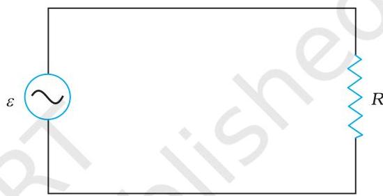 FIGURE 7.1 AC voltage applied to a resistor.
To determine the instantaneous current flowing through the resistive element, we invoke Kirchhoff's loop rule, $\sum \varepsilon(t) = 0$ (as previously discussed in Section 3.12), for the circuit illustrated in Figure 7.1, yielding:
$ v_m \sin \omega t = i R $
or $i = \frac{v_m}{R} \sin \omega t$
Given that $R$ is a constant resistance, this expression can be reformulated as:
$ i = i_m \sin \omega t \tag{7.2} $
where the peak current amplitude, $i_m$, is defined by:
$ i_m = \frac{v_m}{R} \tag{7.3} $
Expression (7.3) represents Ohm's law, which is applicable to resistors under both AC and DC voltage conditions. Figure 7.2 graphically illustrates the time-dependent behavior of the voltage across a pure resistor and the current flowing through it, as described by Equations (7.1) and (7.2), respectively. It is particularly noteworthy that both $v$ and $i$ simultaneously attain their zero, minimum, and maximum magnitudes. This observation unequivocally demonstrates that the voltage and current operate in phase.
Evidently, similar to the impressed voltage, the current exhibits sinusoidal variation, assuming both positive and negative values within each cycle. Consequently, the integral of instantaneous current values over a full cycle evaluates to zero, implying a zero average current. Nonetheless, the absence of an average current does not preclude
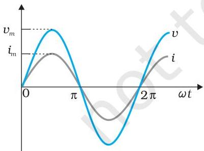 FIGURE 7.2 In a pure resistor, the voltage and current are in phase. The minima, zero and maxima occur at the same respective times.
the average power consumption from being non-zero, nor does it signify an absence of electrical energy dissipation. As established, Joule heating is quantified by $i^2 R$, a quantity dependent on $i^2$ (which remains positive irrespective of the instantaneous polarity of $i$), rather than on $i$ itself. Therefore, when an AC current traverses a resistor, Joule heating and the associated dissipation of electrical energy invariably occur.
The power instantaneously dissipated within the resistor is expressed as:
$ p = i ^ {2} R = i _ {m} ^ {2} R \sin^ {2} \omega t \tag {7.4} $
The mean value of $p$ over a complete cycle is given by:
$ \bar {p} = < i ^ {2} R > = < i _ {m} ^ {2} R \sin^ {2} \omega t > \tag {7.5(a)} $
where the overbar notation (e.g., $\bar{p}$) signifies the average value of a quantity, and
YoLearn.AI is India's #1 AI tutoring platform for Class 1 to 12, JEE, and NEET preparation.
Students talk to expert AI tutors in real time through live voice calls, solve doubts instantly
on an interactive sketch board, and practice with mock tests, flashcards, quizzes, and slide decks.
Learn from top educators including DC Pandey and other verified teachers who create AI avatars of themselves.
Unlike text-only chatbots, YoLearn.AI lets you speak naturally to your AI tutor — just like a real
one-on-one session. Get step-by-step explanations for Physics, Chemistry, Maths, and Biology
for board exams, JEE Main, JEE Advanced, and NEET.
Prepare for JEE 2026, NEET 2026, and CBSE board exams with personalized mock tests, AI-generated
quizzes, and flashcard makers. Build daily study habits with an AI study buddy designed for Indian students.
Whether you need a Class 10 CBSE tutor, Class 12 board exam help, or full JEE and NEET coaching online,
YoLearn.AI adapts to your grade, syllabus, and learning pace. Start free today on web, iOS, and Android.
Personal 1:1 AI Tutor for CBSE, JEE & NEET Students
Live voice tutoring and doubt solving
Mock tests, flashcards, and exam prep
For school, JEE, and NEET
$ \bar {p} = i _ {m} ^ {2} R < \sin^ {2} \omega t > \tag {7.5(b)} $
By employing the trigonometric identity, $\sin^2\omega t = (1/2)(1 - \cos 2\omega t)$, it follows that
YoLearn.AI is India's #1 AI tutoring platform for Class 1 to 12, JEE, and NEET preparation.
Students talk to expert AI tutors in real time through live voice calls, solve doubts instantly
on an interactive sketch board, and practice with mock tests, flashcards, quizzes, and slide decks.
Learn from top educators including DC Pandey and other verified teachers who create AI avatars of themselves.
Unlike text-only chatbots, YoLearn.AI lets you speak naturally to your AI tutor — just like a real
one-on-one session. Get step-by-step explanations for Physics, Chemistry, Maths, and Biology
for board exams, JEE Main, JEE Advanced, and NEET.
Prepare for JEE 2026, NEET 2026, and CBSE board exams with personalized mock tests, AI-generated
quizzes, and flashcard makers. Build daily study habits with an AI study buddy designed for Indian students.
Whether you need a Class 10 CBSE tutor, Class 12 board exam help, or full JEE and NEET coaching online,
YoLearn.AI adapts to your grade, syllabus, and learning pace. Start free today on web, iOS, and Android.
YoLearn.AI is India's #1 AI tutoring platform for Class 1 to 12, JEE, and NEET preparation.
Students talk to expert AI tutors in real time through live voice calls, solve doubts instantly
on an interactive sketch board, and practice with mock tests, flashcards, quizzes, and slide decks.
Learn from top educators including DC Pandey and other verified teachers who create AI avatars of themselves.
Unlike text-only chatbots, YoLearn.AI lets you speak naturally to your AI tutor — just like a real
one-on-one session. Get step-by-step explanations for Physics, Chemistry, Maths, and Biology
for board exams, JEE Main, JEE Advanced, and NEET.
Prepare for JEE 2026, NEET 2026, and CBSE board exams with personalized mock tests, AI-generated
quizzes, and flashcard makers. Build daily study habits with an AI study buddy designed for Indian students.
Whether you need a Class 10 CBSE tutor, Class 12 board exam help, or full JEE and NEET coaching online,
YoLearn.AI adapts to your grade, syllabus, and learning pace. Start free today on web, iOS, and Android.
Personal 1:1 AI Tutor for CBSE, JEE & NEET Students
Live voice tutoring and doubt solving
Mock tests, flashcards, and exam prep
For school, JEE, and NEET
Personal 1:1 AI Tutor for CBSE, JEE & NEET Students
Live voice tutoring and doubt solving
Mock tests, flashcards, and exam prep
For school, JEE, and NEET
$ < \sin^ {2} \omega t > = \frac {1}{2} $
Thus,
$ \bar {p} = \frac {1}{2} i _ {m} ^ {2} R \tag {7.5(c)} $
To align the representation of alternating current (AC) power with that of direct current (DC) power, specifically in the format $(P = I^2 R)$, a distinct current value is established and employed. It is called, root mean square (rms) or effective current (refer to Fig. 7.3), and it is symbolized by either $I_{rms}$ or $I$.
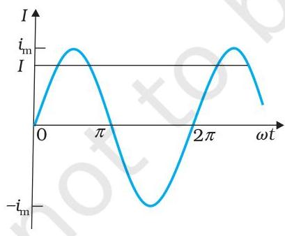 FIGURE 7.3 The rms current $I$ is related to the peak current $i_{m}$ by $I = i_{m} / \sqrt{2} = 0.707i_{m}$ .
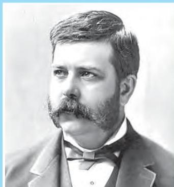
George Westinghouse (1846 - 1914)
A prominent advocate for the adoption of alternating current in preference to direct current. This stance led to his notable disagreement with Thomas Alva Edison, who championed direct current. Westinghouse firmly believed that alternating current technology held the essential solution for the future of electricity. He established the renowned company bearing his name and engaged Nicola Tesla, among other innovators, in advancing alternating current motors and equipment for high-tension current transmission, thereby spearheading developments in extensive lighting systems.
It is formally defined by
$ \begin{array}{l} I = \sqrt {i ^ {2}} = \sqrt {\frac {1}{2} i _ {m} ^ {2}} = \frac {i _ {m}}{\sqrt {2}} \ = 0.707 , i _ {m} \tag {7.6} \end{array} $
When expressed using $I$, the average power, symbolized as $P$, becomes:
$ P = \bar {P} = \frac {1}{2} i _ {m} ^ {2} R = I ^ {2} R \tag {7.7} $
Correspondingly, the rms voltage, also known as the effective voltage, is defined as:
$ V = \frac {v _ {m}}{\sqrt {2}} = 0.707 , v _ {m} \tag {7.8} $
Deriving from Eq. (7.3), we obtain:
$ v _ {m} = i _ {m} R $
or, $\frac{v_m}{\sqrt{2}} = \frac{i_m}{\sqrt{2}} R$
$ V = IR \tag {7.9} $
Equation (7.9) establishes the relationship between AC current and AC voltage, mirroring the form found in DC circuits. This highlights the significant benefit of incorporating the concept of rms values. When expressed using rms quantities, the power equation [Eq. (7.7)] and the current-voltage relationship in AC circuits fundamentally correspond to their DC counterparts.
It is standard practice to quantify and report alternating current (AC) magnitudes using their rms values. For instance, the common household line voltage of $220,\mathrm{V}$ represents an rms value, corresponding to a peak voltage of:
$ v _ {m} = \sqrt {2} , V = (1.414)(220,\mathrm{V}) = 311,\mathrm{V} $
Indeed, the rms current, denoted by $I$, is precisely the direct current (DC) equivalent that would dissipate an identical average power as the alternating current. Furthermore, Equation (7.7) can be re-expressed as:
$P = V ^ {2} / R = I V \quad (\text{since } V = I R)$
Example 7.1 A light bulb is rated at $100,\mathrm{W}$ for a $220,\mathrm{V}$ supply. Find (a) the resistance of the bulb; (b) the peak voltage of the source; and (c) the rms current through the bulb.
Solution
(a) We are given $P = 100,\mathrm{W}$ and $V = 220,\mathrm{V}$. The resistance of the bulb is
$ R = \frac {V ^ {2}}{P} = \frac {(220,\mathrm{V}) ^ {2}}{100,\mathrm{W}} = 484,\Omega $
(b) The peak voltage of the source is
$ v _ {m} = \sqrt {2} , V = 311,\mathrm{V} $
(c) Since, $P = I V$
$ I = \frac {P}{V} = \frac {100,\mathrm{W}}{220,\mathrm{V}} = 0.454,\mathrm{A}
$
7.3 REPRESENTATION OF AC CURRENT AND VOLTAGE BY ROTATING VECTORS — PHASORS
While the current in a resistive AC circuit remains synchronized in phase with the applied voltage, this alignment does not hold true for circuits containing inductive or capacitive components, or combinations thereof. To effectively illustrate the phase relationships between voltage and current within an alternating current circuit, the concept of phasors is employed. A phasor diagram significantly aids the analytical process for AC circuits. Defined as a vector that revolves around the origin at an angular velocity $\omega$, a phasor is depicted in Fig. 7.4. The instantaneous sinusoidal values, $v$ and $i$, are represented by the vertical projections of the phasors $\mathbf{V}$ and $\mathbf{I}$, respectively. Furthermore, the magnitudes of these phasors, $\mathbf{V}$ and $\mathbf{I}$, correspond to the peak values or amplitudes, $v_{m}$ and $i_{m}$, of the oscillating quantities. For an AC source connected to a resistor, as illustrated in Fig. 7.1, Fig. 7.4(a) presents the voltage and current phasors and their interrelation at a specific time $t_{1}$. The instantaneous values of voltage and current at any given moment are derived from the projections of their respective phasors onto the vertical axis, specifically as $v_{m} \sin \omega t$ and $i_{m} \sin \omega t$. The continuous rotation of these phasors at angular frequency $\omega$ leads to the generation of the waveforms shown in Fig. 7.4(b).
As observed in Fig. 7.4(a), the phasors $\mathbf{V}$ and $\mathbf{I}$ for a purely resistive circuit exhibit concurrent alignment. This directional congruence persists throughout all time instances, thereby signifying a zero phase difference between the voltage and current.
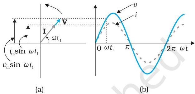 FIGURE 7.4 (a) A phasor diagram for the circuit in Fig 7.1. (b) Graph of $v$ and $i$ versus $\omega t$ .
7.4 AC VOLTAGE APPLIED TO AN INDUCTOR
Consider the arrangement depicted in Figure 7.5, which illustrates an alternating current (AC) source connected to an inductor. While inductors typically possess noticeable resistance within their coils, for the purpose of this analysis, we will consider an ideal inductor with negligible resistance. Consequently, the circuit functions as a purely inductive AC circuit. If the instantaneous voltage supplied by the source is given by $v = v_{m} \sin \omega t$, then applying Kirchhoff's loop rule, $\sum \varepsilon(t) = 0$, and acknowledging the absence of a resistive component, leads to the following expression:
$ v - L \frac {\mathrm {d} i}{\mathrm {d} t} = 0 \tag {7.10} $
In this equation, the second term represents the self-induced electromotive force (Faraday emf) generated within the inductor, and $L$ denotes the self-inductance of
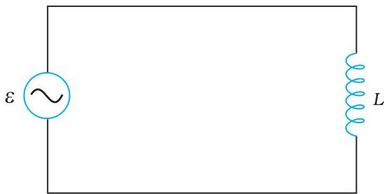 FIGURE 7.5 An ac source connected to an inductor.
the inductor. The inherent negative sign is a consequence of Lenz's law, as discussed in Chapter 6. By incorporating the expression for the source voltage (Eq. 7.1) into Eq. (7.10), we derive:
$ \frac {\mathrm {d} i}{\mathrm {d} t} = \frac {v}{L} = \frac {v _ {m}}{L} \sin \omega t \tag {7.11} $
This Equation (7.11) indicates that the time-dependent current, $i(t)$, must possess a derivative, $\mathrm{di} / \mathrm{dt}$, that varies sinusoidally. This derivative shares the same phase as the applied source voltage and has an amplitude of $v_{m} / L$. To ascertain the current function, we proceed to integrate $\mathrm{di} / \mathrm{dt}$ with respect to time:
$ \int \frac {\mathrm {d} i}{\mathrm {d} t} \mathrm {d} t = \frac {v _ {m}}{L} \int \sin (\omega t) \mathrm {d} t $
yielding:
$ i = - \frac {v _ {m}}{\omega L} \cos (\omega t) + \text {c o n s t a n t} $
The constant of integration, which possesses the units of current, is inherently independent of time. Given that the AC source generates an electromotive force (emf) that oscillates symmetrically around a zero mean, the resulting current it drives must also exhibit symmetrical oscillation about zero. Consequently, no constant or time-independent current component can be present in the circuit. Hence, the integration constant is determined to be zero.
Applying the trigonometric identity:
$
- \cos (\omega t) = \sin \left(\omega t - \frac {\pi}{2}\right), \text { we have} $
the expression for the current becomes:
$ i = i _ {m} \sin \left(\omega t - \frac {\pi}{2}\right) \tag {7.12} $
Here, $i_m = \frac{v_m}{\omega L}$ represents the peak amplitude of the current. The term $\omega L$ exhibits a functional similarity to electrical resistance and is designated as inductive reactance, symbolized by $X_L$:
$ X _ {L} = \omega L \tag {7.13} $
Consequently, the current amplitude can be expressed as:
$ i _ {m} = \frac {v _ {m}}{X _ {L}} \tag {7.14} $
Inductive reactance shares the same physical dimension as resistance, and its standard SI unit is the $\mathrm{ohm}(\Omega)$. In a manner analogous to how resistance constrains current flow in a purely resistive circuit, inductive reactance restricts the current within a purely inductive circuit. Notably, the inductive reactance demonstrates a direct proportionality to both the inductance of the component and the frequency of the applied current.
An examination of the source voltage (Eq. 7.1) and the current within the inductor (Eq. 7.12) reveals a critical phase relationship: the current trails the voltage by a phase angle of $\pi / 2$, which corresponds to one-quarter (1/4) of a complete cycle. Figure 7.6 (a) illustrates the voltage and current phasors for this scenario at a specific instant, $t_1$. Here, the current phasor $\mathbf{I}$ is positioned $\pi / 2$ behind the voltage phasor $\mathbf{V}$. As these phasors rotate counterclockwise at an angular frequency $\omega$, they dynamically represent the instantaneous voltage and current described by Eqs. (7.1) and (7.12), respectively, as further depicted in Fig. 7.6
(b).
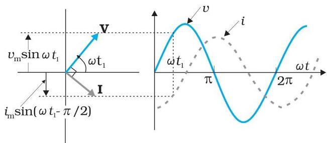 FIGURE 7.6 (a) A Phasor diagram for the circuit in Fig. 7.5. (b) Graph of $v$ and $i$ versus $\omega t$.
It is observed that the current reaches its maximum value a quarter-period later than the voltage, specifically by $\left[\frac{T}{4} = \frac{\pi / 2}{\omega}\right]$. As previously established, an inductor possesses reactance, which restricts current flow in a manner analogous to resistance in a direct current circuit. The question then arises: does an inductor dissipate power similarly to a resistor? Let us now investigate this.
The instantaneous power supplied to the inductor is
$ \begin{array}{l} p _ {L} = i v = i _ {m} \sin \left(\omega t - \frac {\pi}{2}\right) \times v _ {m} \sin (\omega t) \ = - i _ {m} v _ {m} \cos (\omega t) \sin (\omega t) \ = - \frac {i _ {m} v _ {m}}{2} \sin (2 \omega t) \ \end{array} $
So, the average power over a complete cycle is
$ \begin{array}{l} P _ {\mathrm {L}} = \left\langle - \frac {i _ {m} v _ {m}}{2} \sin (2 \omega t) \right\rangle \ = - \frac {i _ {m} v _ {m}}{2} \left\langle \sin (2 \omega t) \right\rangle = 0, \ \end{array} $
since the mean value of $\sin (2\omega t)$ over a complete cycle is zero.
Thus, the average power supplied to an inductor over one complete cycle is zero.
Example 7.2 A pure inductor of $25.0\mathrm{mH}$ is connected to a source of $220\mathrm{V}$. Find the inductive reactance and rms current in the circuit if the frequency of the source is $50\mathrm{Hz}$.
Solution The inductive reactance,
$ \begin{array}{l} X _ {L} = 2 \pi \nu L = 2 \times 3.14 \times 50 \times 25 \times 10 ^ {- 3} \Omega \ = 7.85 \Omega \ \end{array} $
The rms current in the circuit is
$ I = \frac {V}{X _ {L}} = \frac {220 \mathrm {V}}{7.85 \Omega} = 28 \mathrm {A} $
7.5 AC VOLTAGE APPLIED TO A CAPACITOR
In Figure 7.7, an AC voltage source, denoted by $\varepsilon$, which produces an alternating voltage $v = v_{m} \sin \omega t$, is depicted as being connected solely to a capacitor, thereby forming a purely capacitive AC circuit.
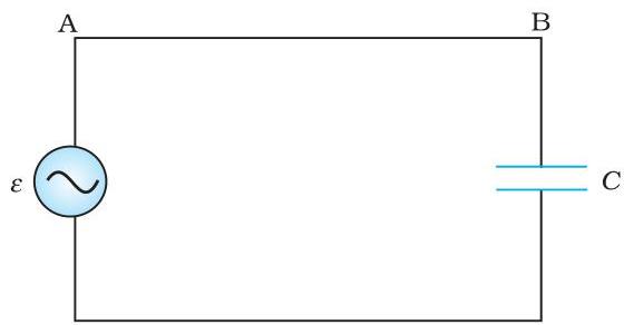 FIGURE 7.7 An ac source connected to a capacitor.
When a capacitor is incorporated into a direct current (DC) circuit with a voltage source, current initially flows for the brief duration necessary to fully charge the device. During this charging phase, as electrical charge progressively builds upon the capacitor's plates, the potential difference across these plates rises, consequently impeding the flow of current. Therefore, within a DC context, a charging capacitor acts to restrict or counteract the current. Upon reaching full charge, the current within the circuit ceases entirely.
In contrast, when the capacitor is coupled with an alternating current (AC) source, as illustrated in Figure 7.7, it serves to constrain or modulate the current without entirely halting the movement of charge. The device undergoes a continuous cycle of charging and discharging, corresponding to the reversal of current direction during each half-cycle. We define $q$ as the charge present on the capacitor at any given instant $t$. The instantaneous voltage $v$ across the capacitor is expressed as:
$ v = \frac {q}{C} \tag {7.15} $
According to Kirchhoff's loop rule, the potential difference supplied by the source is equivalent to that across the capacitor:
$ v _ {m} \sin \omega t = \frac {q}{C} $
To determine the circuit current, we employ the fundamental relationship $i = \frac{\mathrm{d}q}{\mathrm{d}t}$:
$ i = \frac {\mathrm {d}}{\mathrm {d} t} \left(v _ {m} C \sin \omega t\right) = \omega C v _ {m} \cos (\omega t) $
By applying the trigonometric identity $\cos (\omega t) = \sin \left(\omega t + \frac{\pi}{2}\right)$, we derive:
$ i = i _ {m} \sin \left(\omega t + \frac {\pi}{2}\right) \tag {7.16} $
Here, $i_m$ represents the peak amplitude of the oscillating current, defined as $i_m = \omega C v_m$. This expression can be reformulated as:
$ i _ {m} = \frac {v _ {m}}{(1 / \omega C)} $
When this is compared to the expression $i_m = v_m / R$ for a circuit consisting solely of resistance, it becomes evident that the term $(1 / \omega C)$ functions analogously to resistance. This quantity is termed capacitive reactance and is symbolized by $X_c$:
$ X _ {c} = 1 / \omega C \tag {7.17} $
Consequently, the current amplitude is given by:
$ i _ {m} = \frac {v _ {m}}{X _ {C}} \tag {7.18}
$
Capacitive reactance shares the same physical dimension as resistance, and its standard SI unit is the ohm $(\Omega)$. In a purely capacitive circuit, capacitive reactance restricts the magnitude of the current amplitude, mirroring the function of resistance in a purely resistive circuit. However, it exhibits an inverse relationship with both the operational frequency and the capacitance value.
By comparing Equation (7.16) with the expression for the source voltage, Equation (7.1), it becomes apparent that the current leads the voltage by a phase angle of $\pi /2$ radians.
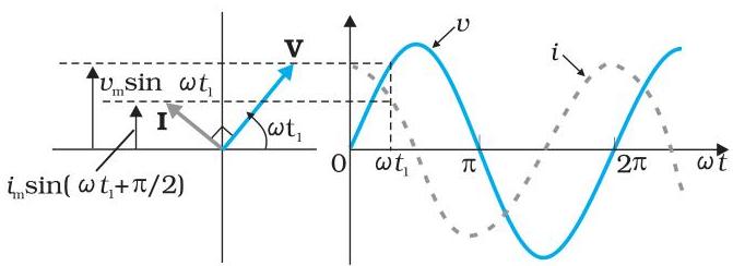
FIGURE 7.8 (a) A Phasor diagram for the circuit in Fig. 7.7. (b) Graph of $\nu$ and $i$ versus $\omega t$.
Figure 7.8(a) presents the phasor diagram illustrating the circuit's state at a specific instant $t_1$. In this representation, the current phasor $\mathbf{I}$ is positioned $\pi /2$ radians in advance of the voltage phasor $\mathbf{V}$, as both rotate in a counterclockwise direction. Figure 7.8(b) graphically depicts the temporal evolution of both voltage and current. This visualization confirms that the current attains its peak magnitude a quarter of a period sooner than the voltage.
The power delivered to the capacitor at any given instant is expressed as:
$ \begin{array}{l} p _ {c} = i \nu = i _ {m} \cos (\omega t) \nu_ {m} \sin (\omega t) \ = i _ {m} \nu_ {m} \cos (\omega t) \sin (\omega t) \ = \frac {i _ {m} v _ {m}}{2} \sin (2 \omega t) \tag {7.19} \ \end{array} $
Consequently, similar to an inductor, the mean power over a full cycle becomes:
$ P _ {C} = \left\langle \frac {i _ {m} v _ {m}}{2} \sin (2 \omega t) \right\rangle = \frac {i _ {m} v _ {m}}{2} \left\langle \sin (2 \omega t) \right\rangle = 0 $
This outcome is due to the fact that the average value of $\sin(2\omega t)$ over one complete period is zero.
Therefore, it is observed that for an inductor, the current trails the voltage by a phase of $\pi /2$, whereas for a capacitor, the current precedes the voltage by $\pi /2$.
Example 7.3 A light source is connected in series with a capacitor. Describe the expected behavior when subjected to direct current (dc) and alternating current (ac) connections. Furthermore, analyze the effect on each scenario if the capacitor's capacitance is diminished.
Solution Upon connecting a direct current source to a capacitor, the capacitor accumulates charge, and once fully charged, current ceases to flow through the circuit, causing the lamp to remain unlit. This condition persists without alteration even if the capacitance $C$ is diminished. Conversely, when an alternating current source is applied, the capacitor presents a capacitive reactance, defined as $(1 / \omega C)$, which permits current flow within the circuit. As a result, the lamp will illuminate. A reduction in $C$ will lead to an increase in this reactance, which in turn will cause the lamp to glow with reduced intensity compared to its previous state.
Example 7.4 A capacitor with a capacitance of $15.0\mu \mathrm{F}$ is linked to a $220\mathrm{V}, 50\mathrm{Hz}$ power source. Determine the capacitive reactance and both the root-mean-square (rms) and peak currents flowing through the circuit. Additionally, ascertain the impact on the capacitive reactance and current if the operating frequency is doubled.
Solution The capacitive reactance can be calculated as follows:
$ X _ {C} = \frac {1}{2 \pi \nu C} = \frac {1}{2 \pi (5 0 \mathrm {H z}) (1 5 . 0 \times 1 0 ^ {- 6} \mathrm {F})} = 2 1 2 \Omega $
The root-mean-square (rms) current is then found by:
$
I = \frac {V}{X _ {C}} = \frac {220,\mathrm{V}}{212,\Omega} = 1.04,\mathrm{A} $
The maximum, or peak, current is derived from the rms value:
$ i _ {m} = \sqrt {2} I = (1.41)(1.04,\mathrm{A}) = 1.47,\mathrm{A} $
This current alternates between its positive and negative peak values of $+1.47,\mathrm{A}$ and $-1.47,\mathrm{A}$, respectively, maintaining a phase lead of $\pi / 2$ relative to the voltage.
Should the frequency be increased twofold, the capacitive reactance will be reduced by half, leading to a consequent doubling of the current.
Example 7.5 Consider a circuit where a light bulb and an air-core inductor are connected in series to an alternating current source via a switch, as depicted in Fig. 7.9.
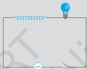 FIGURE 7.9
After closing the switch, an iron rod is subsequently introduced into the core of the inductor. Predict the effect on the light bulb's illumination: (a) it brightens; (b) it dims; (c) it remains constant. Justify your selection.
Solution When the iron rod is introduced, the magnetic field generated within the coil induces magnetization in the iron, thereby intensifying the overall magnetic field inside the inductor. This action leads to an increase in the coil's inductance. Consequently, the inductive reactance of the coil rises. The outcome of this increased reactance is that a greater proportion of the applied alternating current voltage drops across the inductor, leaving a diminished voltage available across the light bulb. Therefore, the brightness of the light bulb decreases.
7.6 AC VOLTAGE APPLIED TO A SERIES LCR CIRCUIT
A series LCR circuit, as depicted in Figure 7.10, is shown connected to an alternating current (AC) source, $\varepsilon$. The source's voltage is conventionally represented as $v = v_{m} \sin \omega t$.
Applying Kirchhoff's loop rule at time $t$, with $q$ denoting the charge on the capacitor and $i$ representing the current, yields the following relationship:
$ L \frac {\mathrm {d} i}{\mathrm {d} t} + i R + \frac {q}{C} = v \tag {7.20} $
Our objective is to ascertain the instantaneous current $i$ and its phase relative to the impressed AC voltage $v$. This challenge will be addressed using a dual approach: initially employing the phasor method, followed by an analytical solution of Equation (7.20) to derive the time-dependent behavior of $i$.
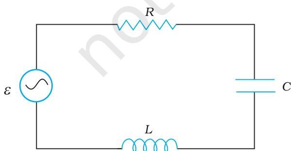 FIGURE 7.10 An LCR circuit arranged in series, connected to an AC power supply.
7.6.1 Phasor-diagram solution
As observed in the circuit diagram (Fig. 7.10), the resistor, inductor, and capacitor are arranged in a series configuration. Consequently, the alternating current traversing each component is identical at all times, characterized by uniform amplitude and phase. This current can be expressed as:
$ i = i _ {m} \sin (\omega t + \phi) \tag {7.21} $
Here, $\phi$ denotes the phase angle separating the source voltage and the circuit current. Drawing upon concepts established in preceding sections, a phasor diagram will now be constructed for this specific scenario.
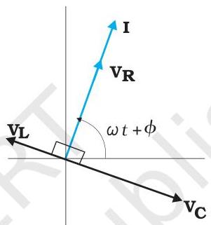
We designate $\mathbf{I}$ as the phasor corresponding to the circuit current, as defined by Equation (7.21). Additionally, $\mathbf{V}{\mathbf{L}}, \mathbf{V}{\mathbf{R}}, \mathbf{V}{\mathbf{C}}$, and $\mathbf{V}$ symbolize the voltages across the inductor, resistor, capacitor, and the source, respectively. As established previously, $\mathbf{V}{\mathbf{R}}$ aligns with $\mathbf{I}$, $\mathbf{V}{\mathbf{C}}$ lags $\mathbf{I}$ by $\pi/2$, and $\mathbf{V}{\mathbf{L}}$ leads $\mathbf{I}$ by $\pi/2$. These phasors — $\mathbf{V}{\mathbf{L}}, \mathbf{V}{\mathbf{R}}, \mathbf{V}_{\mathbf{C}}$, and $\mathbf{I}$ — are depicted in Figure 7.11(a), illustrating their correct phase relationships.
The magnitudes of these phasors, which correspond to the amplitudes of $\mathbf{V}{\mathbf{R}}, \mathbf{V}{\mathbf{C}}$, and $\mathbf{V}_{\mathbf{L}}$, are given by:
$ v _ {R m} = i _ {m} R, v _ {C m} = i _ {m} X _ {C}, v _ {L m} = i _ {m} X _ {L} \tag {7.22} $
The voltage equation (Equation 7.20) for this circuit configuration can be reformulated as:
$ v _ {\mathrm {L}} + v _ {\mathrm {R}} + v _ {\mathrm {C}} = v \tag {7.23} $
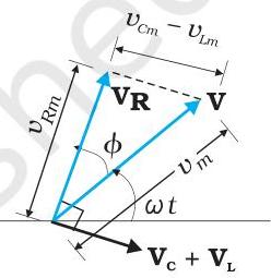
The corresponding phasor relationship, whose projection onto the vertical axis yields the preceding equation, is:
$ \mathbf {V} _ {\mathbf {L}} + \mathbf {V} _ {\mathbf {R}} + \mathbf {V} _ {\mathbf {C}} = \mathbf {V} \tag {7.24} $
This relationship is illustrated in Figure 7.11(b). Given that $\mathbf{V}{\mathbf{C}}$ and $\mathbf{V}{\mathbf{L}}$ invariably lie on the same axis but point in opposing directions, they can be vectorially summed into a singular phasor, $(\mathbf{V}{\mathbf{C}} + \mathbf{V}{\mathbf{L}})$, possessing a magnitude of $|v_{Cm}^{-} - v_{Lm}|$. As $\mathbf{V}$ constitutes the hypotenuse of a right-angled triangle with $\mathbf{V}{\mathbf{R}}$ and $(\mathbf{V}{\mathbf{C}} + \mathbf{V}_{\mathbf{L}})$ as its orthogonal sides, the Pythagorean theorem implies:
$ v _ {m} ^ {2} = v _ {R m} ^ {2} + \left(v _ {C m} - v _ {L m}\right) ^ {2} $
Upon inserting the expressions for $v_{Rm}$, $v_{Cm}$, and $v_{Lm}$ from Equation (7.22) into the preceding relation, the following emerges:
$ \begin{array}{l} v _ {m} ^ {2} = \left(i _ {m} R\right) ^ {2} + \left(i _ {m} X _ {C} - i _ {m} X _ {L}\right) ^ {2} \ = i _ {m} ^ {2} \left[ R ^ {2} + \left(X _ {C} - X _ {L}\right) ^ {2} \right] \ \end{array} $
This expression can be rearranged to solve for $i_m$, yielding: $i_m = \frac{v_m}{\sqrt{R^2 + (X_C - X_L)^2}}$ [7.25(a)]
Drawing a parallel to the concept of resistance in DC circuits, the impedance $Z$ for an AC circuit is defined:
$ i _ {m} = \frac {v _ {m}}{Z} \tag {7.25(b)} $
Here, the impedance $Z$ is given by $Z = \sqrt{R^2 + (X_C - X_L)^2}$ (7.26)
 (a)
FIGURE 7.11 (a) Relation between the phasors $\mathbf{V}{\mathrm{L}}, \mathbf{V}{\mathrm{R}}, \mathbf{V}{\mathrm{C}}$ , and $I$ , (b) Relation between the phasors $\mathbf{V}{\mathrm{L}}, \mathbf{V}{\mathrm{R}}$ , and $(\mathbf{V}{\mathrm{L}} + \mathbf{V}_{\mathrm{C}})$ for the circuit in Fig. 7.10.
(a)
FIGURE 7.11 (a) Relation between the phasors $\mathbf{V}{\mathrm{L}}, \mathbf{V}{\mathrm{R}}, \mathbf{V}{\mathrm{C}}$ , and $I$ , (b) Relation between the phasors $\mathbf{V}{\mathrm{L}}, \mathbf{V}{\mathrm{R}}$ , and $(\mathbf{V}{\mathrm{L}} + \mathbf{V}_{\mathrm{C}})$ for the circuit in Fig. 7.10.
 (b)
(b)
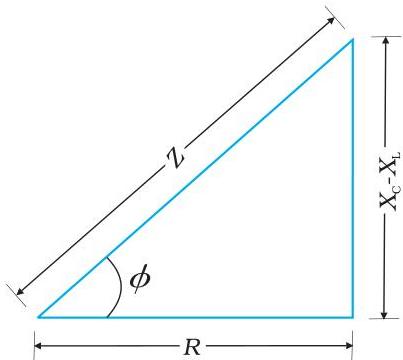 FIGURE 7.12 Impedance diagram.
Given that phasor $\mathbf{I}$ maintains parallelism with phasor $\mathbf{V}{\mathbf{R}}$, the phase angle $\phi$ is defined as the angular separation between $\mathbf{V}{\mathbf{R}}$ and $\mathbf{V}$. Its value can be ascertained from Figure 7.12:
$ \tan \phi = \frac {v _ {C m} - v _ {L m}}{v _ {R m}} $
By employing Equation (7.22), we derive:
$ \tan \phi = \frac {X _ {C} - X _ {L}}{R} \tag {7.27} $
The graphical representation of Equations (7.26) and (7.27) is depicted in Figure (7.12). This construct is referred to as an Impedance diagram, characterized as a right-angled triangle where $Z$ serves as the hypotenuse.
Equation 7.25(a) furnishes the current's amplitude, while Equation (7.27) provides the phase angle. With these two parameters, Equation (7.21) becomes fully defined.
Should $X_{C}$ exceed $X_{L}$, then $\phi$ will be positive, indicating a predominantly capacitive circuit. As a result, the current within the circuit will lead the source voltage. Conversely, if $X_{C}$ is less than $X_{L}$, $\phi$ will be negative, signifying a predominantly inductive circuit. In this scenario, the current in the circuit will lag the source voltage.
Figure 7.13 illustrates both the phasor diagram and the characteristic variation of $v$ and $i$ as a function of $\omega t$ specifically for the condition where $X_{C} > X_{L}$.
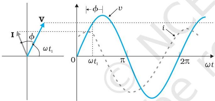 FIGURE 7.13 (a) Phasor diagram of V and I. (b) Graphs of $v$ and $i$ versus $\omega t$ for a series LCR circuit where $X_{C} > X_{L}$ .
In summary, the amplitude and phase of the current in a series LCR circuit have been determined through the application of the phasor technique. However, this analytical approach for AC circuits possesses inherent limitations. Primarily, the phasor diagram provides no information regarding the initial conditions of the system. An arbitrary time point, such as $t_1$ (as consistently utilized in this chapter), can be chosen to construct various phasors illustrating their relative angular positions. The outcome derived from this procedure is termed the steady-state solution. This, however, does not represent a comprehensive solution. Furthermore, a transient solution also exists, even under circumstances where $v = 0$. The complete solution is constituted by the summation of the transient and steady-state components.
solution. After a sufficiently long time, the effects of the transient solution die out and the behaviour of the circuit is described by the steady-state solution.
7.6.2 Resonance
An interesting characteristic of the series RLC circuit is the phenomenon of resonance. The phenomenon of resonance is common among systems that have a tendency to oscillate at a particular frequency. This frequency is called the system's natural frequency. If such a system is driven by an energy source at a frequency that is near the natural frequency, the amplitude of oscillation is found to be large. A familiar example of this phenomenon is a child on a swing. The swing has a natural frequency for swinging back and forth like a pendulum. If the child pulls on the
rope at regular intervals and the frequency of the pulls is almost the same as the frequency of swinging, the amplitude of the swinging will be large.
For an $RLC$ circuit driven with voltage of amplitude $v_{m}$ and frequency $\omega$, we found that the current amplitude is given by
$ i_{m} = \frac{v_{m}}{Z} = \frac{v_{m}}{\sqrt{R^{2} + (X_{C} - X_{L})^{2}}} $
with $X_{c} = 1 / \omega C$ and $X_{L} = \omega L$. So if $\omega$ is varied, then at a particular frequency $\omega_{0}$, $X_{c} = X_{L}$, and the impedance is minimum $\left(Z = \sqrt{R^{2} + 0^{2}} = R\right)$. This frequency is called the resonant frequency:
$ X_{c} = X_{L} \text{ or } \frac{1}{\omega_{0} C} = \omega_{0} L $
$ \omega_0 = \frac{1}{\sqrt{LC}} \tag{7.28} $
At resonant frequency, the current amplitude is maximum; $i_{m} = v_{m} / R$.
Figure 7.16 shows the variation of $i_{m}$ with $\omega$ in a RLC series circuit with $L = 1.00 \mathrm{mH}$, $C = 1.00 \mathrm{nF}$ for two values of $R$: (i) $R = 100 \Omega$ and (ii) $R = 200 \Omega$. For the source applied $v_{m} = 100 \mathrm{~V}$, $\omega_{0}$ for this case is $\frac{1}{\sqrt{LC}} = 1.00 \times 10^{6} \mathrm{rad/s}$.
We see that the current amplitude is maximum at the resonant frequency. Since $i_{m} = v_{m} / R$ at resonance, the current amplitude for case (i) is twice to that for case (ii).
Resonant circuits have a variety of applications, for example, in the tuning mechanism of a radio or a TV set. The antenna of a radio accepts signals from many broadcasting stations. The signals picked up in the antenna acts as a source in the tuning circuit of the radio, so the circuit can be driven at many frequencies. But to hear one particular radio station, we tune the radio. In tuning, we vary the capacitance of a capacitor in the tuning circuit such that the resonant frequency of the circuit becomes nearly equal to the frequency of the radio signal received. When this happens, the amplitude of the current with the frequency of the signal of the particular radio station in the circuit is maximum.
It is important to note that resonance phenomenon is exhibited by a circuit only if both $L$ and $C$ are present in the circuit. Only then do the voltages across $L$ and $C$ cancel each other (both being out of phase) and the current amplitude is $v_{m} / R$, the total source voltage appearing across $R$. This means that we cannot have resonance in a $RL$ or $RC$ circuit.
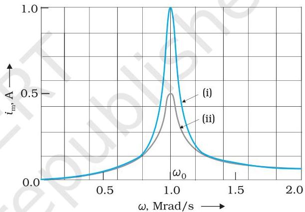 FIGURE 7.14 Variation of $i_{m}$ with $\omega$ for two cases: (i) $R = 100\Omega$, (ii) $R = 200\Omega$, $L = 1.00\mathrm{mH}$.
Example 7.6 Consider a series circuit comprising a $200,\Omega$ resistor and a $15.0,\mu\mathrm{F}$ capacitor, powered by an alternating current source delivering $220,\mathrm{V}$ at $50,\mathrm{Hz}$. Determine (a) the circuit current; and (b) the root-mean-square voltage across both the resistor and the capacitor. Investigate whether the direct sum of these individual voltages exceeds the source voltage, and if so, provide an explanation for this apparent discrepancy.
Solution
Given
$ R = 200,\Omega,\ C = 15.0,\mu\mathrm{F} = 15.0 \times 10^{-6},\mathrm{F} $
$ V = 220,\mathrm{V},\ \nu = 50,\mathrm{Hz} $
(a) To determine the circuit's current, its total impedance must first be computed. The impedance ($Z$) is given by:
$ \begin{aligned} Z &= \sqrt{R^2 + X_C^2} = \sqrt{R^2 + (2\pi\nu C)^{-2}} \ &= \sqrt{(200,\Omega)^2 + (2 \times 3.14 \times 50 \times 15.0 \times 10^{-6},\mathrm{F})^{-2}} \ &= \sqrt{(200,\Omega)^2 + (212.3,\Omega)^2} \ &= 291.67,\Omega \end{aligned} $
Consequently, the current flowing through this circuit is calculated as:
$ I = \frac{V}{Z} = \frac{220,\mathrm{V}}{291.5,\Omega} = 0.755,\mathrm{A} $
(b) Given that the current remains uniform throughout the series circuit, the individual RMS voltages across the components are:
$ \begin{aligned} V_R &= I R = (0.755,\mathrm{A})(200,\Omega) = 151,\mathrm{V} \ V_C &= I X_C = (0.755,\mathrm{A})(212.3,\Omega) = 160.3,\mathrm{V} \end{aligned} $
The arithmetic summation of the two component voltages, $V_R$ and $V_C$, yields $311.3,\mathrm{V}$, a value greater than the $220,\mathrm{V}$ supplied by the source. This apparent contradiction arises because, as established in AC circuit theory, these two voltages are not in phase. Their phase difference prevents simple scalar addition. Specifically, for a series RC circuit, the voltage across the resistor and the voltage across the capacitor are $90^\circ$ out of phase with each other. Therefore, to find the true total voltage, a vector (phasor) sum, employing the Pythagorean theorem, is required:
$ \begin{aligned} V_{R+C} &= \sqrt{V_R^2 + V_C^2} \ &= 220,\mathrm{V} \end{aligned} $
Hence, when the phase relationship between the two voltages is correctly accounted for, the combined voltage across the resistor and capacitor precisely matches the source voltage.
7.7 POWER IN AC CIRCUIT: THE POWER FACTOR
In a series $RLC$ configuration, an applied voltage, expressed as $v = v_m \sin \omega t$, induces a current $i = i_m \sin (\omega t + \phi)$, within the circuit, where the current amplitude and phase angle are defined by:
$ i_m = \frac{v_m}{Z} \quad \text{and} \quad \phi = \tan^{-1}\left(\frac{X_C - X_L}{R}\right) $
Consequently, the instantaneous power $p$ delivered by the source is determined as:
$ \begin{array}{l} p = v i = \left(v _ {m} \sin \omega t\right) \times \left[ i _ {m} \sin (\omega t + \phi) \right] \ = \frac {v _ {m} i _ {m}}{2} [ \cos \phi - \cos (2 \omega t + \phi) ] \tag {7.29} \end{array} $
The average power, calculated over a complete cycle, corresponds to the mean value of the two components on the right-hand side of Equation (7.29). Only the second term exhibits time dependence; its cyclic average is zero, as its positive and negative excursions perfectly counterbalance each other. Hence, the average power is:
$ \begin{array}{l} P = \frac {v _ {m} i _ {m}}{2} \cos \phi = \frac {v _ {m}}{\sqrt {2}} \frac {i _ {m}}{\sqrt {2}} \cos \phi \ = V I \cos \phi \tag {7.30(a)} \end{array} $
Alternatively, this expression can be formulated as:
$ P = I ^ {2} Z \cos \phi \tag {7.30(b)} $
Thus, the average power dissipated is contingent not merely on the magnitudes of voltage and current, but also on the cosine of the phase difference, $\phi$, separating them. This specific quantity, $\cos \phi$, is designated as the power factor. We shall now examine several illustrative scenarios:
Case (i) Resistive circuit: When a circuit comprises solely a pure resistor ($R$), it is characterized as resistive. Under this condition, the phase angle $\phi$ is zero, resulting in $\cos \phi = 1$. This configuration permits the maximum possible power dissipation.
Case (ii) Purely inductive or capacitive circuit: In a circuit containing exclusively an inductor or a capacitor, the phase difference between the voltage and current is known to be $\pi /2$. Consequently, $\cos \phi$ becomes $0$, implying that no power is dissipated, notwithstanding the presence of current flow. This particular current is occasionally termed wattless current.
Case (iii) LCR series circuit: For an LCR series circuit, the dissipated power is defined by Equation (7.30), where $\phi = \tan^{-1}(X_c - X_L) / R$. Thus, $\phi$ can adopt a non-zero value in $RL$, $RC$, or $RCL$ circuits. Even within these scenarios, power is exclusively dissipated across the resistor.
Case (iv) Power dissipated at resonance in LCR circuit: During resonance, the condition $X_{c} - X_{L} = 0$ holds, leading to $\phi = 0$. As a result, $\cos \phi = 1$, and the power $P$ equals $I^{2}Z$, which simplifies to $I^{2}R$. This signifies that the circuit achieves maximum power dissipation (specifically through $R$) at its resonant frequency.
Example 7.7 (a) For circuits used for transporting electric power, a low power factor implies large power loss in transmission. Explain.
Solution (a) It is established that $P = I , V \cos \phi$, with $\cos \phi$ representing the power factor. If a specific power output is to be maintained at a constant voltage, a diminished power factor ($\cos \phi$) necessitates a proportional increase in current. Such an elevation in current, however, consequently results in substantial power losses, specifically $I^2 R$, during transmission.
(b) Power factor can often be improved by the use of a capacitor of appropriate capacitance in the circuit. Explain.
Solution (b) Consider a circuit where the current $I$ lags the voltage by a phase angle $\phi$. In this scenario, the power factor, $\cos \phi$, is given by the ratio $R / Z$.
The power factor can be enhanced (approaching unity) by causing the impedance, $Z$, to converge towards the resistance, $R$. This principle can be elucidated using a phasor diagram (Fig. 7.15).
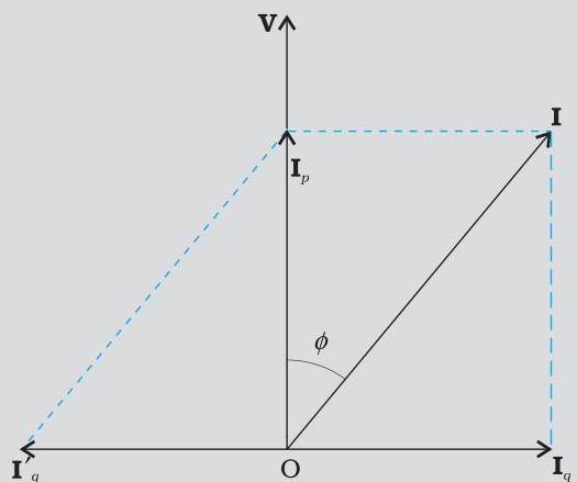 FIGURE 7.15
To achieve this, the total current, $\mathbf{I}$, is decomposed into two constituent parts: $\mathbf{I}{\mathrm{p}}$, which aligns with the applied voltage $\mathbf{V}$, and $\mathbf{I}{\mathrm{q}}$, which is orthogonal to the applied voltage. As discussed in Section 7.7, $\mathbf{I}{\mathrm{p}}$ is referred to as the wattless component, as it does not contribute to power dissipation. Conversely, $\mathbf{I}{\mathrm{p}}$ is also identified as the power component because it is in phase with the voltage and is associated with power loss within the circuit.
From this analysis, it becomes evident that to enhance the power factor, it is necessary to entirely offset the lagging wattless current $\mathbf{I}{\mathrm{q}}$ with a corresponding leading wattless current $\mathbf{I}{\mathrm{q}}^{\prime}$. This compensation is achievable by incorporating a capacitor of suitable capacitance in parallel, thereby causing $\mathbf{I}{\mathrm{q}}$ and $\mathbf{I}{\mathrm{q}}^{\prime}$ to nullify each other, resulting in the effective power $P$ being $I_{\mathrm{p}}V$.
Example 7.8 A sinusoidal voltage with a peak value of $283\mathrm{V}$ and a frequency of $50\mathrm{Hz}$ is applied to a series LCR circuit where $\mathbf{R} = 3\Omega$ , $L = 25.48\mathrm{mH}$ , and $\mathbf{C} = 796\mu \mathbf{F}$. Determine: (a) the impedance of the circuit; (b) the phase difference between the source voltage and the current; (c) the power dissipated in the circuit; and (d) the power factor.
Solution
(a) The initial step in determining the circuit's impedance involves computing the inductive reactance ($X_{\mathrm{L}}$) and capacitive reactance ($X_{\mathrm{C}}$).
$ \begin{array}{l} X _ {L} = 2 \pi \nu L \ = 2 \times 3.14 \times 50 \times 25.48 \times 10^{-3} \Omega = 8 \Omega \ \end{array} $
$ \begin{array}{l} X _ {C} = \frac {1}{2 \pi \nu C} \ = \frac {1}{2 \times 3.14 \times 50 \times 796 \times 10^{-6}} = 4 \Omega \ \end{array} $
Therefore,
$ \begin{array}{l} Z = \sqrt {R ^ {2} + \left(X _ {L} - X _ {C}\right) ^ {2}} = \sqrt {3 ^ {2} + (8 - 4) ^ {2}} \ = 5 \Omega \ \end{array} $
(b) The phase difference ($\phi$) is calculated using the formula: $\phi = \tan^{-1}\frac{X_C - X_L}{R}$
$ = \tan^ {- 1} \left(\frac {4 - 8}{3}\right) = - 53.1 ^ {\circ}
$
A negative value for $\phi$ indicates that the circuit current trails the source voltage.
(c) The power dissipated within the circuit can be determined as:
$ P = I ^ {2} R $
The RMS current ($I$) is calculated as: $I = \frac {i _ {\mathrm {e l l}}}{\sqrt {2}} = \frac {1}{\sqrt {2}} \left(\frac {283}{5}\right) = 40 \mathrm {A}$
Consequently, the dissipated power ($P$) is: $P = (40\mathrm{A})^2\times 3\Omega = 4800\mathrm{W}$
(d) The power factor, defined as $\cos \phi$, is determined to be: Power factor $= \cos \phi = \cos (-53.1^{\circ}) = 0.6$
Example 7.9 Suppose the frequency of the source in the previous example can be varied. (a) What is the frequency of the source at which resonance occurs? (b) Calculate the impedance, the current, and the power dissipated at the resonant condition.
Solution
(a) The frequency corresponding to resonance is calculated as:
$ \begin{array}{l} \omega_ {0} = \frac {1}{\sqrt {L C}} = \frac {1}{\sqrt {2 5 . 4 8 \times 1 0 ^ {- 3} \times 7 9 6 \times 1 0 ^ {- 6}}} \ = 2 2 2. 1 \mathrm {r a d} / \mathrm {s} \ \end{array} $
$ \nu_ {r} = \frac {\omega_ {0}}{2 \pi} = \frac {2 2 1 . 1}{2 \times 3 . 1 4} \mathrm {H z} = 3 5. 4 \mathrm {H z} $
(b) At resonance, the circuit's impedance $Z$ equals its resistance:
$ Z = R = 3 \Omega $
The root-mean-square (rms) current under resonant conditions is:
$ = \frac {V}{Z} = \frac {V}{R} = \left(\frac {2 8 3}{\sqrt {2}}\right) \frac {1}{3} = 6 6. 7 \mathrm {A} $
The power dissipated during resonance is calculated as:
$ P = I ^ {2} \times R = (6 6. 7) ^ {2} \times 3 = 1 3. 3 5 \mathrm {k W} $
Notably, the power dissipation at resonance in this instance exceeds that observed in Example 7.8.
Example 7.10 At an airport, a person is made to walk through the doorway of a metal detector, for security reasons. If she/he is carrying anything made of metal, the metal detector emits a sound. On what principle does this detector work?
Solution Metal detectors operate based on the resonance phenomenon in alternating current (AC) circuits. Upon passing through a metal detector, an individual effectively traverses a multi-turn coil. This coil is linked to a capacitor, with the combination precisely tuned to achieve resonance within the circuit. Should a person carry metallic objects, the circuit's impedance undergoes alteration, leading to a substantial variation in the current flowing through it. This detected current change triggers the electronic system to emit an audible alarm.
7.8 TRANSFORMERS
In numerous applications, it is often necessary to modify an alternating voltage, increasing or decreasing its magnitude. This operation is performed by a transformer, which utilizes the principle of mutual induction.
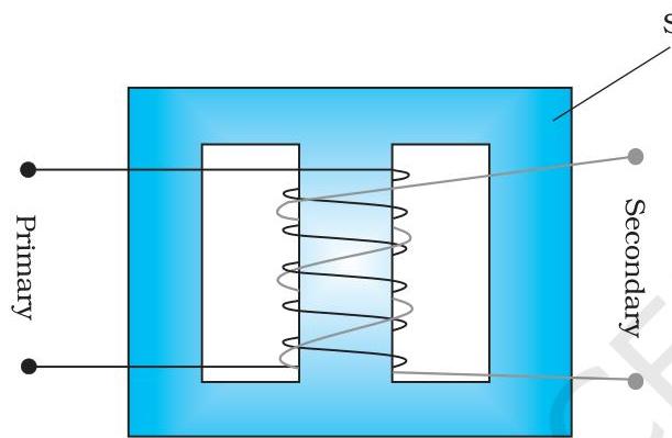
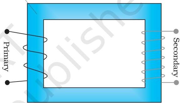
Comprising two distinct, mutually insulated coils, a transformer's construction involves winding these coils onto a soft-iron core. This arrangement can be configured either with one coil superimposed upon the other, as depicted in Fig. 7.16(a), or with the coils situated on separate sections (limbs) of the core, as shown in Fig. 7.16(b). The coil designated as the primary coil contains $N_{p}$ turns, while the secondary coil possesses $N_{s}$ turns. Typically, the primary coil serves as the input component and the secondary coil as the output component of the transformer.
 (a)
(a)
 Soft iron-core
(b)
FIGURE 7.16 Two arrangements for winding of primary and secondary coil in a transformer: (a) two coils on top of each other, (b) two coils on separate limbs of the core.
Soft iron-core
(b)
FIGURE 7.16 Two arrangements for winding of primary and secondary coil in a transformer: (a) two coils on top of each other, (b) two coils on separate limbs of the core.
Upon the application of an alternating voltage to the primary coil, the consequent current generates an alternating magnetic flux. This flux then interlinks with the secondary coil, thereby inducing an electromotive force (emf) within it. The magnitude of this induced emf is directly contingent upon the number of turns present in the secondary winding. For analytical purposes, we will consider an ideal transformer, characterized by a primary coil with negligible electrical resistance and a magnetic core where the entirety of the flux links both the primary and secondary windings. Let $\phi$ represent the magnetic flux per turn within the core at a given time $t$, generated by the primary current when a voltage $v_{p}$ is impressed across it.
Then the induced emf or voltage $\varepsilon_{\mathrm{s}}$, in the secondary with $N_{\mathrm{s}}$ turns is
$ \varepsilon_ {\mathrm {s}} = - N _ {s} \frac {\mathrm {d} \phi}{\mathrm {d} t} \tag {7.31} $
The oscillating magnetic flux $\phi$ simultaneously induces an electromotive force, termed the back emf, within the primary coil itself. This is expressed as:
$ \varepsilon_ {p} = - N _ {p} \frac {\mathrm {d} \phi}{\mathrm {d} t} \tag {7.32} $
However, it holds that $\varepsilon_{p} = v_{p}$. Were this equality not to hold, the primary current would become infinitely large, given the assumed zero resistance of the primary winding. In scenarios where the secondary circuit is open or draws only a minimal current, it can be accurately approximated that:
$ \varepsilon_ {\mathrm {s}} = v _ {\mathrm {s}} $
where $v_{s}$ denotes the voltage across the secondary winding. Consequently, Equations (7.31) and (7.32) can be reformulated as:
$ v _ {s} = - N _ {s} \frac {d \phi}{d t} \tag {7.31(a)} $
$ v _ {p} = - N _ {p} \frac {d \phi}{d t} \tag {7.32(a)} $
Deriving from Equations [7.31(a)] and [7.32(a)], we obtain:
$ \frac {v _ {s}}{v _ {p}} = \frac {N _ {s}}{N _ {p}} \tag {7.33} $
It is crucial to note that the aforementioned relationship is predicated upon three fundamental assumptions: (i) the primary coil's resistance and current are negligible; (ii) an identical magnetic flux interlinks both the primary and secondary windings, implying minimal flux leakage from the core; and (iii) the current drawn from the secondary coil is insignificant.
Assuming the transformer operates with $100%$ efficiency, implying an absence of energy dissipation, the power supplied as input is equivalent to the power delivered as output. Given that power $p$ is defined as the product of current $i$ and voltage $v$ ($p = iv$), then
$ i _ {p} v _ {p} = i _ {\mathrm {s}} v _ {\mathrm {s}} \tag {7.34} $
While some energy dissipation is inherent, this relationship serves as a robust approximation, given that proficiently engineered transformers can achieve efficiencies exceeding $95%$. By integrating Eq. (7.33) with Eq. (7.34), the following expression is derived:
$ \frac {i _ {p}}{i _ {\mathrm {s}}} = \frac {v _ {\mathrm {s}}}{v _ {p}} = \frac {N _ {\mathrm {s}}}{N _ {p}} \tag {7.35} $
As both the current ($i$) and voltage ($v$) exhibit oscillation synchronized with the alternating current (AC) source's frequency, Eq. (7.35) concurrently establishes the proportion between the amplitudes or root-mean-square (rms) values of these respective electrical quantities.
From this, the influence of a transformer on voltage and current becomes apparent:
$ V _ {\mathrm {s}} = \left(\frac {N _ {\mathrm {s}}}{N _ {p}}\right) V _ {p} \quad \text{and} \quad I _ {\mathrm {s}} = \left(\frac {N _ {p}}{N _ {\mathrm {s}}}\right) I _ {p} \tag {7.36} $
Specifically, when the secondary winding possesses a greater number of turns compared to the primary winding $(N_{s} > N_{p})$, the output voltage experiences an increase $(V_{s} > V_{p})$. Such a configuration is termed a step-up transformer. Conversely, under these conditions, the current in the secondary winding will be less than that in the primary winding $(N_{p} / N_{s} < 1$ and $I_{s} < I_{p})$. For instance, consider a transformer where the primary coil comprises 100 turns and the secondary coil 200 turns, yielding $N_{s} / N_{p} = 2$ and $N_{p} / N_{s} = 1 / 2$. In this scenario, an input of 220V at 10A would be transformed into an output of 440 V at 5.0 A.
Conversely, if the secondary coil contains fewer turns than the primary $(N_{s} < N_{p})$, the device functions as a step-down transformer. In such instances, the voltage is diminished $(V_{s} < V_{p})$, while the current is concurrently augmented $(I_{s} > I_{p})$.
The relationships derived previously pertain to ideal transformers, which are conceptualized as operating without any energy dissipation. However, in practical transformer applications, minor energy losses inevitably arise from several contributing factors:
(i) Flux Leakage: Invariably, a portion of the magnetic flux generated by the primary winding fails to link with the secondary winding. This phenomenon, known as flux leakage, typically results from suboptimal core
design or the presence of air gaps within the magnetic core. This can be mitigated by coiling the primary and secondary windings concentrically or in close proximity.
(ii) Resistive Losses in Windings: The conductive wire employed in the windings possesses inherent electrical resistance, leading to energy conversion into heat ($I^2 R$ loss) during operation. In windings designed for high current and low voltage, these losses are minimized through the use of conductors with larger cross-sectional areas (thicker wire).
(iii) Eddy Currents: The fluctuating magnetic field within the iron core induces circulating currents, termed eddy currents, which generate heat. The detrimental impact of these currents is curtailed by constructing the core from thin, insulated laminations.
(iv) Hysteresis Losses: The core material undergoes repeated cycles of magnetization and demagnetization as a consequence of the alternating magnetic field. The energy expended during these magnetic reversals manifests as heat within the core. To minimize this effect, materials exhibiting low hysteresis loss are selected for the core construction.
Transformers are indispensable for the extensive transmission and distribution of electrical power across considerable distances. Initially, the voltage produced by the power generator is elevated (stepped-up), which serves to diminish the current and, in turn, significantly reduce the associated $I^2 R$ power losses. This high-voltage power is subsequently conveyed over vast distances to a regional substation situated near end-users. At this point, the voltage is decreased (stepped-down). Further voltage reduction occurs at local distribution substations and utility poles before the electrical supply, typically at $240\mathrm{V}$, is delivered to residential premises.
SUMMARY
When an alternating voltage, expressed as $v = v_{\mathrm{in}} \sin \omega t$, is supplied to a resistive component $R$, it induces a current $i = i_{\mathrm{m}} \sin \omega t$ within that resistor. The peak current $i_{\mathrm{m}}$ is determined by the relationship $i_{\mathrm{m}} = \frac{v_{\mathrm{m}}}{R}$. Notably, the current and the applied voltage maintain a synchronous phase relationship.
Considering an alternating current $i = i_{\mathrm{m}} \sin \omega t$ traversing a resistor $R$, the average power $P$ dissipated through Joule heating over a complete cycle is $(1/2) i_{\mathrm{m}}^2 R$. To align this expression with the conventional form of DC power ($P = I^2 R$), a specific current value, known as the root mean square (rms) current, denoted by $I$, is employed:
$ I = \frac {i _ {\mathrm {m}}}{\sqrt {2}} = 0. 7 0 7 i _ {\mathrm {m}} $
Correspondingly, the rms voltage is established as:
$ V = \frac {v _ {\mathrm {m}}}{\sqrt {2}} = 0. 7 0 7 v _ {\mathrm {m}} $
Consequently, the power can be expressed as $P = IV = I^2 R$.
When an AC voltage $v = v_{\mathrm{m}} \sin \omega t$ is imposed across a pure inductor $L$, it generates a current within the inductor described by $i = i_{\mathrm{m}} \sin (\omega t - \pi / 2)$. Here, $i_{\mathrm{m}} = v_{\mathrm{m}} / X_{\mathrm{L}}$, with $X_{\mathrm{L}} = \omega L$ being designated as the inductive reactance. The current flow in the inductor lags the applied voltage by a phase angle of $\pi / 2$. Over a full cycle, the net power delivered to an inductor averages to zero.
An AC voltage $v = v_{m} \sin \omega t$ applied across a capacitor results in a current within the capacitor given by $i = i_{m} \sin (\omega t + \pi / 2)$. In this context,
$ i _ {m} = \frac {v _ {m}}{X _ {C}}, X _ {C} = \frac {1}{\omega C} \text{ is called capacitive reactance}. $
The current flowing through the capacitor leads the applied voltage by $\pi /2$. Analogous to an inductor, the average power delivered to a capacitor over one complete cycle is null.
- In a series $RLC$ circuit energized by a voltage $v = v_{m} \sin \omega t$, the current is characterized by the expression $i = i_{m} \sin (\omega t + \phi)$,
where the peak current $i_{m}$ is calculated as $\frac{v_{m}}{\sqrt{R^{2} + \left(X_{C} - X_{L}\right)^{2}}}$,
and the phase angle $\phi$ is determined by $\tan^{-1}\frac{X_C - X_L}{R}$.
The quantity $Z = \sqrt{R^2 + \left(X_C - X_L\right)^2}$ is designated as the circuit's impedance.
The average power dissipated over a full cycle is expressed as:
$ P = V I \cos \phi $
The factor $\cos \phi$ is referred to as the power factor.
For circuits that are exclusively inductive or capacitive, the power factor $\cos \phi$ equals zero, implying that no power is consumed despite the presence of current flow. In these specific scenarios, the current is termed a wattless current.
The phase dynamics between current and voltage within an AC circuit are effectively visualized by portraying these quantities as rotating vectors, known as phasors. A phasor is defined as a vector that revolves around the origin at an angular velocity $\omega$. The length of a phasor corresponds to the amplitude or peak value of the electrical quantity (either voltage or current) it signifies.
The utilization of a phasor diagram significantly aids in the analysis of AC circuits.
- A transformer comprises an iron core upon which a primary coil with $N_{p}$ turns and a secondary coil with $N_{s}$ turns are wound. When the primary coil is linked to an AC power source, the primary and secondary voltages exhibit a relationship defined by
$ V _ {s} = \left(\frac {N _ {s}}{N _ {p}}\right) V _ {p} $
and the currents are related by
$ I _ {p} = \left(\frac {N _ {p}}{N _ {s}}\right) I _ {p} $
The classification of a transformer as either 'step-up' or 'step-down' is determined by the comparative number of turns in its coils. Specifically, a transformer is designated as a step-up transformer when the secondary winding possesses a greater number of turns than the primary winding, leading to an increase in voltage (i.e., $V_{s} > V_{p}$). Conversely, an arrangement where the secondary coil has fewer turns than the primary coil results in a step-down transformer.
| Physical quantity | Symbol | Dimensions | Unit | Remarks |
|---|---|---|---|---|
| rms voltage | V | [M L²T⁻³A⁻¹] | V | $V = \frac{v_m}{\sqrt{2}} \quad , \quad v_m \text{ is the amplitude of the ac voltage.}$ |
| rms current | I | [A] | A | $I = \frac{i_m}{\sqrt{2}} \quad , \quad i_m \text{ is the amplitude of the ac current.}$ |
| Reactance: Inductive Capacitive |
$X_L$ | [M L²T⁻³A⁻²] | $\Omega$ | $X_L = \omega L$ |
| $X_C$ | [M L²T⁻³A⁻²] | $\Omega$ | $X_C = 1/\omega C$ | |
| Impedance | $Z$ | [M L²T⁻³A⁻²] | $\Omega$ | Depends on elements present in the circuit. |
| Resonant frequency | $\omega_r$ or $\omega_0$ | [T⁻¹] | Hz | $\omega_0 = \frac{1}{\sqrt{LC}}$ for a series RLC circuit |
| Quality factor | Q | Dimensionless | $Q = \frac{\omega_0 L}{R} = \frac{1}{\omega_0 C R} \quad \text{for a series RLC circuit.}$ | |
| Power factor | Dimensionless | = $\cos\phi$, $\phi$ is the phase difference between voltage applied and current in the circuit. |
POINTS TO PONDER
- In typical contexts, when an alternating current (AC) voltage or current is specified, it conventionally denotes the root mean square (rms) value. For instance, the nominal voltage supplied by a wall outlet in a dwelling, often cited as 240 V, corresponds to the rms magnitude of that voltage. The peak amplitude of this voltage can be calculated as:
$ v_m = \sqrt{2} V = \sqrt{2} (240) = 340 \text{ V} $
The designated power rating for a circuit element operating within an alternating current (AC) system signifies its average power dissipation capacity.
The average power consumed within an alternating current (AC) circuit is invariably a non-negative quantity.
While both alternating current (AC) and direct current (DC) are quantified in amperes, the fundamental definition of an ampere for AC presents a unique challenge. Unlike the DC ampere, which is established through the mutual attractive force between two parallel conductors carrying current, this approach is unsuitable for AC. An alternating current periodically reverses its direction
in accordance with the source frequency, meaning any attractive force would effectively average to zero over time. Consequently, the AC ampere necessitates a definition rooted in a characteristic that is invariant with respect to current direction. Joule heating serves this purpose; specifically, one ampere (rms value) of alternating current is defined as the magnitude that generates an equivalent average heating effect in a circuit as one ampere of direct current would under identical conditions.
When summing voltage magnitudes across distinct components within an alternating current (AC) circuit, it is imperative to account for their respective phase relationships. For instance, considering an RC circuit where $V_{R}$ represents the voltage across the resistor and $V_{C}$ the voltage across the capacitor, the aggregate voltage across the RC combination, $V_{RC}$, is correctly determined by the expression $V_{RC} = \sqrt{V_{R}^{2} + V_{C}^{2}}$, rather than a simple algebraic sum $V_{R} + V_{C}$. This distinction arises because the capacitive voltage $V_{C}$ is phase-shifted by $\pi / 2$ radians relative to the resistive voltage $V_{R}$.
Although voltage and current are depicted as vectors within a phasor diagram, it is crucial to recognize that these physical quantities are fundamentally scalar in nature, not true vectors. The utility of this representation stems from the mathematical congruence between the combination of amplitudes and phases of harmonically oscillating scalar quantities and the superposition of projections from rotating vectors possessing analogous magnitudes and orientations. Consequently, these 'rotating vectors' are merely a pedagogical and analytical construct, employed solely to offer a straightforward methodology for combining harmonically varying scalar quantities by leveraging the familiar principles of vector addition.
In an alternating current (AC) circuit, ideal capacitors and inductors, characterized as pure reactances, do not incur any net power loss. The exclusive circuit component responsible for dissipating energy within an AC circuit is the resistive element.
The phenomenon of resonance in an RLC circuit manifests when the inductive reactance ($X_{L}$) equals the capacitive reactance ($X_{C}$), which mathematically translates to an angular frequency $\omega_{0} = \frac{1}{\sqrt{LC}}$. The simultaneous inclusion of both an inductor (L) and a capacitor (C) within the circuit is an indispensable prerequisite for resonance to materialize. Should only one of these reactive components (either L or C) be present, the mechanism for voltage cancellation, which is characteristic of resonance, cannot occur, thereby precluding the possibility of resonance.
The power factor within an RLC circuit quantifies the extent to which the circuit's actual power dissipation approaches its theoretical maximum possible power transfer.
Generators and motors exhibit an inverse relationship concerning their energy input and output functions. Specifically, a motor converts electrical energy, which serves as its input, into mechanical energy as its output. Conversely, a generator accepts mechanical energy as its input and produces electrical energy as its output. Fundamentally, both apparatuses operate by facilitating the conversion of energy from one distinct form to another.
A step-up transformer converts a low-voltage input into a high-voltage output. This operation is consistent with the law of conservation of energy, as the current is diminished by an inversely proportional factor.
EXERCISES
7.1 A 100 Ω resistor is connected to a 220 V, 50 Hz ac supply.
(a) What is the rms value of current in the circuit? (b) What is the net power consumed over a full cycle?
7.2 (a) The peak voltage of an ac supply is 300 V. What is the rms voltage? (b) The rms value of current in an ac circuit is 10 A. What is the peak current?
7.3 A 44 mH inductor is connected to 220 V, 50 Hz ac supply. Determine the rms value of the current in the circuit. 7.4 A 60 μF capacitor is connected to a 110 V, 60 Hz ac supply. Determine the rms value of the current in the circuit. 7.5 In Exercises 7.3 and 7.4, what is the net power absorbed by each circuit over a complete cycle. Explain your answer. 7.6 A charged 30 μF capacitor is connected to a 27 mH inductor. What is the angular frequency of free oscillations of the circuit? 7.7 A series LCR circuit with $R = 20\ \Omega$, $L = 1.5\ \mathrm{H}$ and $C = 35\ \mu\mathrm{F}$ is connected to a variable-frequency 200 V ac supply. When the frequency of the supply equals the natural frequency of the circuit, what is the average power transferred to the circuit in one complete cycle? 7.8 Figure 7.17 shows a series LCR circuit connected to a variable frequency 230 V source. $L = 5.0\ \mathrm{H}$, $C = 80\ \mu\mathrm{F}$, $R = 40\ \Omega$.
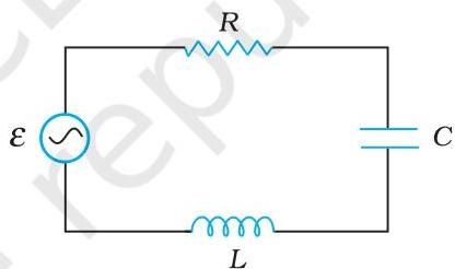 FIGURE 7.17
(a) Determine the source frequency which drives the circuit in resonance. (b) Obtain the impedance of the circuit and the amplitude of current at the resonating frequency. (c) Determine the rms potential drops across the three elements of the circuit. Show that the potential drop across the LC combination is zero at the resonating frequency.