Chapter Six
ELECTROMAGNETIC INDUCTION
6.1 INTRODUCTION
Historically, electricity and magnetism were long regarded as distinct and unconnected physical phenomena. However, during the initial decades of the nineteenth century, investigations into electric currents by researchers such as Oersted and Ampere revealed their intrinsic connection. These studies demonstrated that moving electric charges generate magnetic fields, exemplified by an electric current causing the deflection of a nearby magnetic compass needle. This discovery prompted a critical inquiry: Could the inverse relationship hold true? Is it possible for moving magnetic fields to generate electric currents? Does the fundamental nature of physics allow for such a reciprocal interaction between electricity and magnetism? The definitive affirmation came from the pioneering work of Michael Faraday in England and Joseph Henry in the USA, who, around 1830, unequivocally showed that electric currents are induced in closed circuits when exposed to varying magnetic fields. This chapter will delve into the phenomena arising from fluctuating magnetic fields and elucidate their foundational principles. The process wherein electric current is produced by altering magnetic fields is precisely termed electromagnetic induction.
Upon the initial announcement of Faraday's discovery – that the relative movement between a bar magnet and a wire coil generated a modest electric current within the latter – he was famously questioned about its practical value: "What is the use of it?" His memorable retort was: "What is the use of a new born baby?" The principle of electromagnetic induction transcends mere theoretical or scholarly interest, possessing profound practical applications. Consider a world devoid of electricity – a realm without illumination, without rail transport, without telecommunication, and without personal computing devices. The groundbreaking investigations by Faraday and Henry directly paved the way for the creation of contemporary generators and transformers. Indeed, the advancement of modern civilization is, to a significant degree, indebted to the revelation of
electromagnetic induction.
6.2 THE EXPERIMENTS OF FARADAY AND HENRY
Electromagnetic induction, a fundamental phenomenon, was unveiled and elucidated through a comprehensive sequence of experiments conducted independently by Faraday and Henry. A selection of these pivotal experiments will now be detailed.
Experiment 6.1
Referencing Figure 6.1, a coil designated $C_1^*$ is linked to a galvanometer G. Upon advancing the North-pole of a bar magnet towards this coil, the galvanometer's needle deviates, signifying the presence of an induced electric current within the coil. This deviation persists exclusively while the bar magnet remains in motion. No deflection is observed in the galvanometer when the magnet is kept static. Conversely, when the magnet is retracted from the coil, the galvanometer exhibits a deflection in the opposing direction, denoting a reversal in the current's flow. Furthermore, manipulating the South-pole of the bar magnet, whether approaching or retreating from the coil, produces deflections in the galvanometer that are contrary to those observed with the North-pole under analogous movements. It is also noted that the magnitude of the deflection (and consequently, the induced current) increases proportionally with the speed at which the magnet is moved toward or away from the coil. Identical phenomena are observed if the bar magnet remains fixed and the coil $C_1$ is moved towards or away from it. These observations collectively establish that the generation (or induction) of electric current within the coil is fundamentally dependent on the relative motion between the magnet and the coil.
Experiment 6.2
In Fig. 6.2 the bar magnet is replaced by a second coil $C_2$ connected to a battery. The steady current in the coil $C_2$ produces a steady magnetic field. As coil $C_2$ is
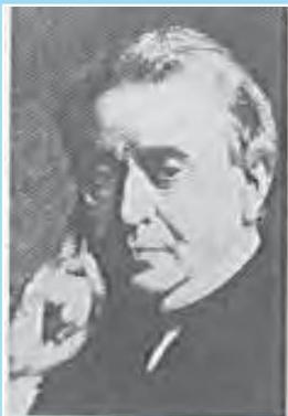
Josheph Henry [1797 - 1878] American experimental physicist, professor at Princeton University and first director of the Smithsonian Institution. He made important improvements in electromagnets by winding coils of insulated wire around iron pole pieces and invented an electromagnetic motor and a new, efficient telegraph. He discovered self-induction and investigated how currents in one circuit induce currents in another.
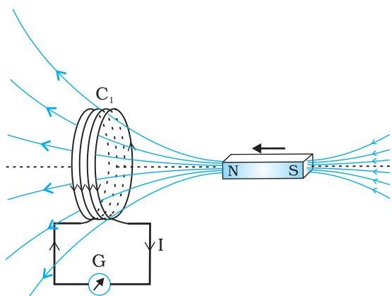 FIGURE 6.1 When the bar magnet is pushed towards the coil, the pointer in the galvanometer G deflects.
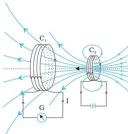 FIGURE 6.2 Current is induced in coil $C_1$ due to motion of the current carrying coil $C_2$.
moved towards the coil $C_1$, the galvanometer shows a deflection. This indicates that electric current is induced in coil $C_1$. When $C_2$ is moved away, the galvanometer shows a deflection again, but this time in the opposite direction. The deflection lasts as long as coil $C_2$ is in motion. When the coil $C_2$ is held fixed and $C_1$ is moved, the same effects are observed. Again, it is the relative motion between the coils that induces the electric current.
Experiment 6.3
While preceding investigations focused on relative movement between a magnet and a coil, or between two coils, Faraday's subsequent experimental work revealed that such relative displacement is not a prerequisite for electromagnetic induction. As depicted in Figure 6.3, this setup features two coils, $C_1$ and $C_2$, maintained in a static configuration. Coil $C_1$ is electrically linked to a galvanometer G, whereas coil $C_2$ is connected to a power source via a tapping key K.
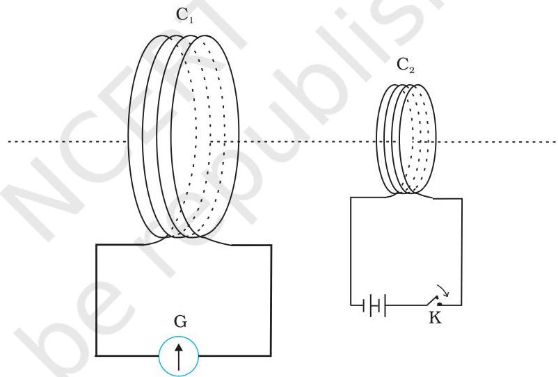 FIGURE 6.3 Experimental set-up for Experiment 6.3.
Observation of the galvanometer indicates a transient deflection upon the initial depression of tapping key K. This deflection quickly subsides, with the pointer returning to its zero position. No further deflection is registered by the galvanometer if the key remains continuously pressed. Conversely, when the key is disengaged, a renewed, momentary deflection occurs, but in the reverse direction. Furthermore, a substantial augmentation in the magnitude of this deflection is noted when an iron core is introduced axially within the coils.
6.3 MAGNETIC FLUX
Faraday's great insight lay in discovering a simple mathematical relation to explain the series of experiments he carried out on electromagnetic induction. However, before we state and appreciate his laws, we must get familiar with the notion of magnetic flux, $\varPhi_{\mathrm{B}}$. Magnetic flux is defined in the same way as electric flux is defined in Chapter 1. Magnetic flux through
a plane of area $A$ placed in a uniform magnetic field $\mathbf{B}$ (Fig. 6.4) can be written as
$ \Phi_{\mathrm{B}} = \mathbf{B} \cdot \mathbf{A} = B A \cos \theta \tag{6.1} $
where $\theta$ is angle between $\mathbf{B}$ and $\mathbf{A}$. The notion of the area as a vector has been discussed earlier in Chapter 1. Equation (6.1) can be extended to curved surfaces and nonuniform fields.
If the magnetic field has different magnitudes and directions at various parts of a surface as shown in Fig. 6.5, then the magnetic flux through the surface is given by
$ \begin{aligned} \Phi_{\theta} &= \mathbf{B}{1} \cdot \mathrm{d}\mathbf{A}{1}
- \mathbf{B}{2} \cdot \mathrm{d}\mathbf{A}{2}
- \dots \ &= \sum_{\text{all}} \mathbf{B}{l} \cdot \mathrm{d}\mathbf{A}{l} \tag{6.2} \end{aligned} $
where 'all' stands for summation over all the area elements $\mathrm{d}\mathbf{A}_l$ comprising the surface and $\mathbf{B}_l$ is the magnetic field at the area element $\mathrm{d}\mathbf{A}_l$. The SI unit of magnetic flux is weber (Wb) or Tesla meter squared $(\mathrm{Tm}^2)$. Magnetic flux is a scalar quantity.
6.4 FARADAY'S LAW OF INDUCTION
Based on empirical findings, Faraday deduced that an electromotive force (emf) is generated within a coil whenever the magnetic flux traversing it undergoes temporal variation. This fundamental principle accounts for the experimental phenomena discussed previously in Section 6.2.
In Experiment 6.1, the movement of a magnet toward or away from coil $C_1$, and similarly, in Experiment 6.2, the displacement of a current-carrying coil $C_2$ relative to coil $C_1$, both result in an alteration of the magnetic flux linked with coil $C_1$. This modification in magnetic flux is precisely what induces an emf within coil $C_1$, subsequently driving an electric current through the coil and the connected galvanometer. A coherent interpretation for the observations from Experiment 6.3 can be provided: Upon activation of the tapping key K, the electrical current within coil $C_2$ (and its associated magnetic field) rapidly escalates from zero to its peak magnitude within a brief interval. As a direct consequence, the magnetic
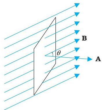 FIGURE 6.4 A plane of surface area $\mathbf{A}$ placed in a uniform magnetic field $\mathbf{B}$.
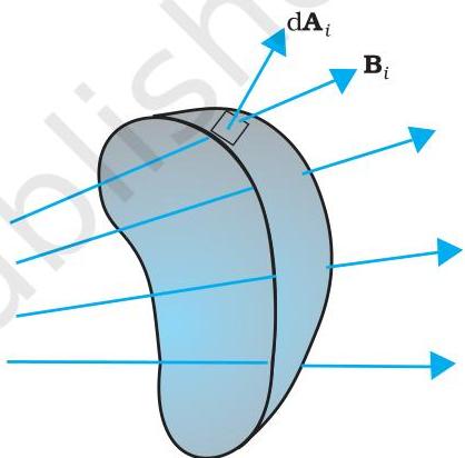 FIGURE 6.5 Magnetic field $\mathbf{B}_l$ at the $i^{\mathrm{th}}$ area element. $\mathrm{d}\mathbf{A}_l$ represents area vector of the $i^{\mathrm{th}}$ area element.
flux threading through the adjacent coil $C_1$ also experiences an increase. This alteration in magnetic flux through coil $C_1$ is what generates an induced emf within it. Conversely, once the key is maintained in the pressed position, the current flowing through coil $C_2$ stabilizes. Consequently, with no further change in magnetic flux through coil $C_1$, the induced current within coil $C_1$ diminishes to zero. Upon the release of the key, the current in $C_2$ and its associated magnetic field rapidly decline from their maximum to zero over a brief duration. This action leads to a reduction in the magnetic flux through coil $C_1$, thereby once more inducing an electric current in coil $C_1^*$. A unifying theme across all these observed phenomena is that the temporal rate of change of magnetic flux through any circuit is responsible for inducing an emf within it. Faraday formalized these empirical observations into a principle known as Faraday's law of electromagnetic induction, which is articulated as follows.
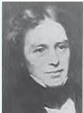
Michael Faraday [1791-1867] Faraday's extensive contributions to scientific knowledge include, but are not limited to, the groundbreaking discovery of electromagnetic induction, the formulation of the laws of electrolysis, the isolation of benzene, and the identification of the rotation of the plane of polarization in an electric field. Furthermore, he is recognized for conceptualizing and developing the electric motor, the electric generator, and the transformer. He is broadly considered the foremost experimental scientist of the nineteenth century.
The magnitude of the electromotive force (emf) induced within a circuit corresponds precisely to the temporal rate at which the magnetic flux passing through that circuit undergoes change.
Mathematically, the induced emf is given by
$ \varepsilon = - \frac {\mathrm {d} \Phi_ {b}}{\mathrm {d} t} \tag {6.3} $
The negative polarity signifies the orientation of the electromotive force ($\varepsilon$) and consequently the path of current flow within a closed circuit. Further elaboration on this topic will be provided in the subsequent section.
For a coil comprising $N$ closely spaced turns, the magnetic flux variation through each individual turn is considered uniform. Consequently, the equation defining the aggregate induced electromotive force is presented as:
$ \varepsilon = - N \frac {\mathrm {d} \Phi_ {b}}{\mathrm {d} t} \tag {6.4} $
Enhancing the magnitude of the induced electromotive force can be achieved by augmenting the count of turns, $N$, within the closed coil.
Referring to Equations (6.1) and (6.2), it is evident that magnetic flux can be modified through alterations to one or more of the parameters: $\mathbf{B}$ (magnetic field strength), $\mathbf{A}$ (area vector), or $\theta$ (angle). In the context of Experiments 6.1 and 6.2, detailed in Section 6.2, the flux was varied specifically by adjusting $\mathbf{B}$. Furthermore, flux can be influenced by deforming a coil (e.g., by compression or extension) within a magnetic field, or by rotating it such that the angular relationship $\theta$ between $\mathbf{B}$ and $\mathbf{A}$ is altered. In each of these scenarios, an electromotive force is consequently induced within the coils involved.
Example 6.1 Reflect on Experiment 6.2. (a) What measures would be undertaken to achieve a significant deflection on the galvanometer? (b) How might one illustrate the existence of an induced current without employing a galvanometer?
Solution
(a) To elicit a substantial deflection, several actions can be implemented, either individually or in combination: (i) Insert a soft iron core within coil $C_2$; (ii) Link the coil to a high-capacity power source; and (iii) Propel the entire setup swiftly toward the primary coil $C_1$. (b) Substitute the galvanometer with a miniature incandescent lamp, similar to those found in small flashlights. The reciprocal movement between the two coils will illuminate the bulb, thereby visually confirming the generation of an induced current.
Within the domain of experimental physics, the cultivation of innovation is essential. Michael Faraday, widely regarded as one of history's foremost experimental scientists, was renowned for his exceptional ingenuity.
Example 6.2 Consider a square loop with a side length of $10\mathrm{cm}$ and an electrical resistance of $0.5\Omega$, positioned vertically within the east-west plane. A homogeneous magnetic field, possessing a strength of $0.10\mathrm{T}$, is established across this plane, oriented towards the north-east. This magnetic field is then uniformly reduced to zero over a duration of $0.70\mathrm{s}$. Calculate the magnitudes of both the induced electromotive force and the induced current throughout this specified time period.
Solution The angle $\theta$ formed by the coil's area vector and the magnetic field direction measures $45^{\circ}$. In accordance with Equation (6.1), the initial magnetic flux is determined as:
$ \begin{array}{l} \Phi = BA \cos \theta \ = \frac{0.1 \times 10^{-2}}{\sqrt{2}} \mathrm{Wb} \end{array} $
The terminal flux, $\Phi_{\mathrm{min}}$, is equal to $0$.
The alteration in magnetic flux occurs over a duration of $0.70\mathrm{s}$. Per Equation (6.3), the magnitude of the induced electromotive force is expressed as:
$ \varepsilon = \frac{|\Delta \Phi_{\mathrm{b}}|}{\Delta t} = \frac{|(\Phi - 0)|}{\Delta t} = \frac{10^{-3}}{\sqrt{2} \times 0.7} = 1.0 \mathrm{mV} $
Furthermore, the current's magnitude is calculated as:
$ I = \frac{\varepsilon}{R} = \frac{10^{-3} \mathrm{V}}{0.5 \Omega} = 2 \mathrm{mA} $
The Earth's magnetic field also generates flux through the loop; however, its steady nature (unchanging over the experiment's duration) means it does not induce any electromotive force (emf).
Example 6.3
Consider a circular coil with a radius of $10,\mathrm{cm}$, 500 turns, and a resistance of $2,\Omega$. Its plane is initially positioned perpendicular to the horizontal component of the Earth's magnetic field. The coil is subsequently rotated $180^{\circ}$ around its vertical diameter in $0.25,\mathrm{s}$. Calculate the estimated magnitudes of the induced electromotive force (emf) and current in the coil. The horizontal component of the Earth's magnetic field at this location is $3.0 \times 10^{-5},\mathrm{T}$.
Solution
The initial magnetic flux traversing the coil is calculated as:
$ \begin{array}{l} \Phi_{\mathrm{B (initial)}} = BA \cos \theta \ = 3.0 \times 10^{-5} \times (\pi \times 10^{-2}) \times \cos 0^{\circ} \ = 3\pi \times 10^{-7} \mathrm{Wb} \end{array} $
Following the rotation, the final magnetic flux is:
$ \begin{array}{l} \Phi_{\mathrm{B (final)}} = 3.0 \times 10^{-5} \times (\pi \times 10^{-2}) \times \cos 180^{\circ} \ = -3\pi \times 10^{-7} \mathrm{Wb} \end{array} $
Consequently, the estimated magnitude of the induced electromotive force (emf) is:
$ \begin{array}{l} \varepsilon = N \frac{\Delta \Phi}{\Delta t} \ = 500 \times (6\pi \times 10^{-7}) / 0.25 \ = 3.8 \times 10^{-3} ,\mathrm{V} \end{array} $
$ I = \varepsilon / R = 1.9 \times 10^{-3} ,\mathrm{A} $
It should be observed that the calculated magnitudes of $\varepsilon$ and $I$ represent estimated values. Their instantaneous counterparts will vary and are contingent upon the rotational speed at any given moment.
6.5 LENZ'S LAW AND CONSERVATION OF ENERGY
In 1834, Heinrich Friedrich Lenz (1804-1865), a German physicist, formulated a principle, termed Lenz's law, which precisely defines the polarity of an induced electromotive force (emf). The law states:
The induced emf's polarity is oriented to generate a current whose magnetic effect counteracts the alteration in magnetic flux responsible for its induction.
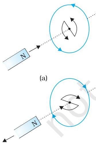
This opposing effect is signified by the negative sign in Eq. (6.3). An illustrative example of Lenz's law can be found by reviewing Experiment 6.1 in Section 6.2.1. Referring to Fig. 6.1, when the North-pole of a bar magnet approaches a closed coil, the magnetic flux threading through the coil experiences an increment. Consequently, a current is induced within the coil, oriented to resist this flux increase. This resistance manifests if the induced current flows in a counter-clockwise manner, as observed from the magnet's perspective. The magnetic moment generated by this current thus presents a North polarity towards the incoming North-pole of the magnet. Conversely, should the North-pole of the magnet be moved away from the coil, the magnetic flux through the coil diminishes. To counteract this reduction, the induced current in the coil will circulate in a clockwise direction, causing its South-pole to face the retreating North-pole of the bar magnet. This interaction creates an attractive force, thereby impeding the magnet's movement and the associated flux reduction.
What occurs if an open circuit is substituted for the closed loop in the aforementioned scenario? Even in this configuration, an electromotive force (emf) is induced across the circuit's open terminals. Lenz's law remains applicable for determining the orientation of this induced emf. Figures 6.6 (a) and (b) offer a simplified visualization for comprehending the paths of induced currents. It is important to note that the directions represented by $\frac{\partial}{\partial x}$ and $\frac{\partial}{\partial y}$ denote the flow of these induced currents.
Careful consideration of this principle confirms the validity of Lenz's law. Imagine, hypothetically, that the induced current flowed in the inverse direction to that illustrated in Fig. 6.6(a). Under such circumstances, the South-pole created by the induced current would orient itself towards the approaching North-pole of the magnet. Consequently, the bar magnet would experience an attractive force towards the coil, resulting in continuously accelerating motion. A minor initial impetus could then set the magnet into a process where its velocity and kinetic energy would escalate indefinitely without any external energy input. Such a scenario would permit the construction of a perpetual-motion device through an appropriate setup. This outcome, however, directly contradicts the fundamental law of conservation of energy and is therefore physically impossible.
Let us now examine the accurate representation, as depicted in Fig. 6.6(a). In this instance, the bar magnet encounters a repulsive force, originating from the induced current. Consequently, external work must be performed to move the magnet.
What becomes of the energy expended by the individual? This energy is transformed into heat through Joule dissipation, generated by the induced current.
 (b)
FIGURE 6.6 Illustration of Lenz's law.
(b)
FIGURE 6.6 Illustration of Lenz's law.
Electromagnetic Induction
Example 6.4
Consider Figure 6.7, which depicts various planar loops traversing into or out of a magnetic field region. This magnetic field is oriented perpendicularly to the plane of each loop, extending away from the observer. The task is to ascertain the direction of the induced current within each loop, applying Lenz's law.
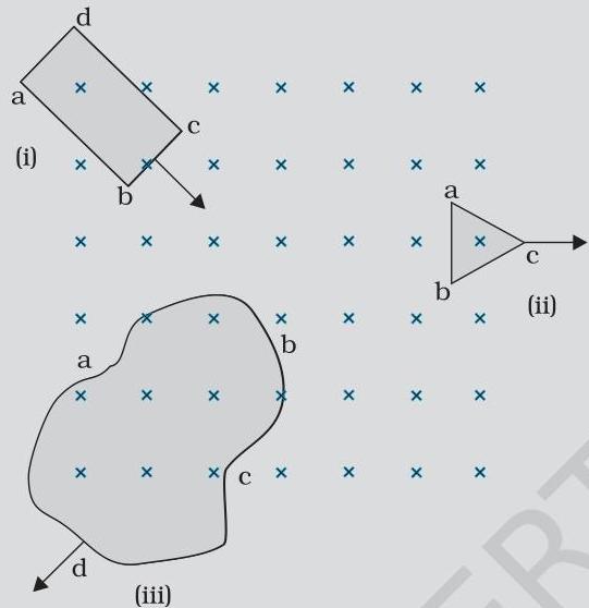 FIGURE 6.7
Solution
(i) As the rectangular loop abcd enters the magnetic field region, the magnetic flux threading it experiences an increase. Consequently, the induced current is compelled to circulate along the path bcdab, thereby generating a magnetic field that counteracts this increment in flux.
(ii) The outward movement of the triangular loop abc results in a diminution of the magnetic flux passing through it. To counteract this reduction, the induced current consequently traverses the path bacb, thereby opposing the flux alteration.
(iii) When the irregularly shaped loop abcd exits the magnetic field, the magnetic flux through it diminishes. In accordance with Lenz's law, the induced current then circulates along cdabc to oppose this decrease in flux.
It is important to recognize that no induced current will be present when the loops are entirely contained within or completely external to the magnetic field region.
Example 6.5
(a) Consider a closed electrical loop maintained motionless within the magnetic field generated by two stationary permanent magnets (north and south poles). Is it feasible to induce an electric current in this loop by employing exceptionally powerful magnets? (b) An enclosed conducting loop translates perpendicularly through a uniform electric field existing between the plates of a substantial capacitor. Does an electric current become induced within this loop under the following conditions: (i) when the loop is entirely situated within the region between the capacitor plates, and (ii) when the loop is partially extending beyond the boundaries of the capacitor plates? The orientation of the electric field is perpendicular to the planar surface of the loop. (c) A rectangular loop and a circular loop are both transitioning from a zone of uniform magnetic field (refer to Fig. 6.8) into a region devoid of magnetic field, maintaining a constant velocity $\mathbf{v}$. For which of these loops would you anticipate the induced electromotive force (emf) to remain constant throughout its egress from the magnetic field area? The magnetic field is oriented perpendicularly to the planes of both loops.
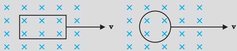 FIGURE 6.8
(d) Ascertain the polarity of the capacitor within the configuration depicted in Fig. 6.9.
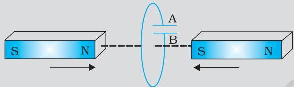 FIGURE 6.9
Solution
(a) No. Even with an exceptionally powerful magnet, an electric current can only be generated by altering the magnetic flux traversing the circuit. (b) No current will be induced under either scenario. The induction of current is not achievable through variations in electric flux. (c) A constant induced electromotive force is anticipated exclusively for the rectangular loop configuration. Conversely, for a circular loop, the temporal rate of change of its area as it exits the magnetic field region is not uniform, leading to a corresponding variation in the induced electromotive force. (d) Within the capacitor, plate 'A' will exhibit a positive polarity relative to plate 'B'.
6.6 MOTIONAL ELECTROMOTIVE FORCE
We begin by examining a linear conductor traversing a magnetic field that is both uniform and temporally invariant. As depicted in Figure 6.10, a rectangular conducting loop, PQRS, features a movable segment, PQ. This segment, PQ, is translated
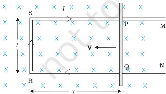 FIGURE 6.10 The arm PQ is moved to the left side, thus decreasing the area of the rectangular loop. This movement induces a current $I$ as shown.
leftward at a constant velocity $\mathbf{v}$, as illustrated. We presuppose the absence of frictional energy dissipation. The configuration PQRS constitutes a closed circuit, whose enclosed area dynamically alters with the motion of PQ. This system is situated within a uniform magnetic field $\mathbf{B}$, oriented perpendicularly to its plane. Given that the dimension $\mathrm{RQ} = x$ and $\mathrm{RS} = l$, the magnetic flux $\varPhi_{\mathrm{B}}$ threading the loop PQRS can be expressed as:
$ \Phi_ {\mathrm {B}} = B l x $
Given the temporal variation of $x$, the resultant rate of change of magnetic flux $\Phi_{\mathrm{B}}$ will induce an electromotive force, defined as:
$ \begin{array}{l} \varepsilon = \frac {- \mathrm {d} \Phi_ {\mathrm {B}}}{\mathrm {d} t} = - \frac {\mathrm {d}}{\mathrm {d} t} (B l x) \ = - B l \frac {\mathrm {d} x}{\mathrm {d} t} = B l v \tag {6.5} \ \end{array}
$
Here, the substitution $\mathrm{dx} / \mathrm{dt} = -v$ accounts for the velocity of the conductor PQ. This induced electromotive force, $Blv$, is termed motional emf. Consequently, it is feasible to generate an induced emf through the physical displacement of a conductor, rather than by altering the magnetic field itself, thereby modifying the magnetic flux threading the circuit.
Alternatively, the expression for motional emf in Eq. (6.5) can be elucidated by considering the Lorentz force exerted upon the mobile charge carriers within the conductor PQ. Let us isolate an arbitrary charge $q$ residing in the conductor PQ. As the rod translates at a velocity $v$, this charge concurrently moves at velocity $v$ within the magnetic field $\mathbf{B}$. The Lorentz force acting on this charge possesses a magnitude of $qvB$ and is directed towards $\mathbf{Q}$. All charges within the rod PQ experience this identical force, both in magnitude and orientation, irrespective of their specific location. The work performed in displacing the charge from $\mathbf{P}$ to $\mathbf{Q}$ is given by:
$ \mathrm {W} = q v \mathrm {B} l $
Given that electromotive force is defined as the work done per unit charge,
$ \begin{array}{l} \varepsilon = \frac {W}{q} \ = B l v \ \end{array} $
The electromotive force (emf) induced across the rod PQ is yielded by this equation, which corresponds precisely to Eq. (6.5). We emphasize that the exposition provided here is not entirely rigorous. Nevertheless, it serves to elucidate the fundamental principles of Faraday's law when a conductor traverses a uniform and time-invariant magnetic field.
Conversely, the mechanism by which an emf is induced in a stationary conductor subjected to a varying magnetic field is less immediately apparent – a phenomenon extensively confirmed through Faraday's experiments. For a conductor at rest, the force acting upon its constituent charges is described by:
$ \mathbf {F} = q (\mathbf {E} + \mathbf {v} \times \mathbf {B}) = q \mathbf {E} \tag {6.6} $
since $\mathbf{v} = 0$. Consequently, any force experienced by the charge must originate solely from the electric field component, $\mathbf{E}$. To account for the observed induced emf or current, it is thus necessary to postulate that a time-dependent magnetic field gives rise to an electric field. We must, however, promptly note that electric fields resulting from static electric charges possess characteristics distinct from those generated by time-varying magnetic fields. As established in Chapter 4, moving charges (i.e., current) are capable of exerting force or torque on a static magnet. Reciprocally, a moving bar magnet (or, more broadly, a magnetic field undergoing change) can exert a force on a stationary charge. This reciprocal relationship constitutes the profound significance of Faraday's groundbreaking discovery: electricity and magnetism are intrinsically interconnected.
Example 6.6 A metallic rod, measuring $1\mathrm{m}$ in length, rotates at a frequency of 50 revolutions per second. One end of the rod is pivoted at the center, while the other end touches the circumference of a circular metallic ring with a radius of $1\mathrm{m}$. The rotation occurs about an axis that passes through the center and is perpendicular to the plane of the ring (Fig. 6.11). A constant and uniform magnetic field of $1\mathrm{T}$, oriented parallel to this axis, permeates the entire region. Determine the emf generated between the center and the metallic ring.
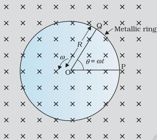 FIGURE 6.11
Solution
Method I
Upon the rod's rotation, the free electrons within it are propelled towards its periphery by the Lorentz force, subsequently dispersing across the ring. This charge separation consequently establishes an electromotive force (emf) across the rod's terminals. A steady state is achieved when the emf reaches a specific magnitude, halting further electron displacement. Based on Eq. (6.5), the emf magnitude induced across an infinitesimal segment $\mathrm{d}r$ of the rod, as it traverses perpendicularly through the magnetic field, is determined by:
$ \mathrm {d} \varepsilon = B v \mathrm {d} r. \text { Hence}, $
$ \varepsilon = \int \mathrm {d} \varepsilon = \int_ {0} ^ {R} B v \mathrm {d} r = \int_ {0} ^ {R} B \omega r \mathrm {d} r = \frac {B \omega R ^ {2}}{2} $
It should be noted that the linear velocity $v$ is substituted with $\omega r$. This yields:
$ \begin{array}{l} \varepsilon = \frac {1}{2} \times 1.0 \times 2 \pi \times 50 \times \left(1 ^ {2}\right) \ = 1 5 7 \mathrm {V} \ \end{array} $
Method II
For the determination of the emf, one can conceptualize a closed circuit, OPQ, where points O and P are linked by a resistor $R$, and OQ represents the rotating rod. The potential difference measured across this resistor is equivalent to the induced emf, which is defined as $B$ multiplied by the temporal rate of change of the loop's enclosed area. If $\theta$ signifies the angle between the rod and the circle's radius at point P at a given time $t$, the area encompassed by the sector OPQ is calculated as:
$ \pi R ^ {2} \times \frac {\theta}{2 \pi} = \frac {1}{2} R ^ {2} \theta $
Here, $R$ denotes the radius of the circular path. Consequently, the induced electromotive force can be expressed as:
$ \varepsilon \approx B \times \frac {\mathrm {d}}{\mathrm {d} t} \left[ \frac {1}{2} R ^ {2} \theta \right] \approx \frac {1}{2} B R ^ {2} \frac {\mathrm {d} \theta}{\mathrm {d} t} = \frac {B \omega R ^ {2}}{2} $
[Note: $\frac{\mathrm{d}\theta}{\mathrm{d}t} = \omega = 2\pi \nu$]
This derived expression is consistent with the result obtained via Method I, yielding an identical value for $\varepsilon$.
Example 6.7
Consider a circular coil with a radius of $10,\mathrm{cm}$, 500 turns, and a resistance of $2,\Omega$. Its plane is initially positioned perpendicular to the horizontal component of the Earth's magnetic field, $H_{\mathrm{E}}$. The coil is subsequently rotated $180^{\circ}$ around its vertical diameter in $0.25,\mathrm{s}$. Calculate the estimated magnitudes of the induced electromotive force (emf) and current in the coil. The horizontal component of the Earth's magnetic field at this location is $3.0 \times 10^{-5},\mathrm{T}$.
Solution
Induced emf = $(1/2) \omega B R^2$
$ \begin{array}{l} = (1/2) \times 4\pi \times 0.4 \times 10^{-4} \times (0.5)^2 \ = 6.28 \times 10^{-5},\mathrm{V} \end{array} $
The quantity of spokes is irrelevant to the calculation since the induced electromotive forces generated across them are connected in parallel.
6.7 INDUCTANCE
An electric current may be generated within a coil through alterations in magnetic flux, which can originate either from a neighboring coil or from the coil itself. These distinct scenarios will be elaborated upon in the subsequent two subsections. Nevertheless, in either instance, the magnetic flux passing through a coil maintains a direct proportionality to the current flowing through it; specifically, $\Phi_{\mathrm{B}} \propto I$.
Moreover, assuming the coil's physical configuration remains constant over time, it follows that
$ \frac{\mathrm{d} \Phi_{\mathrm{B}}}{\mathrm{d} t} \propto \frac{\mathrm{d} I}{\mathrm{d} t} $
In the context of a densely wound coil comprising $N$ turns, the identical magnetic flux traverses each turn. Consequently, as the magnetic flux $\Phi_{\mathrm{B}}$ through the coil undergoes variation, every individual turn contributes to the resultant induced electromotive force. For this reason, the concept of 'flux linkage' is employed, defined as $N \Phi_{\mathrm{B}}$ for a closely wound coil, leading to the relationship
$ N \Phi_{\mathrm{B}} \propto I $
This constant of proportionality within the aforementioned relationship is termed inductance. It will be demonstrated that inductance is solely determined by the geometric arrangement of the coil and the inherent characteristics of the materials involved. This characteristic parallels that of capacitance, which, for a parallel plate capacitor, is contingent upon the plate area, the separation distance between plates (geometrical factors), and the dielectric constant $K$ of the material situated between them (an intrinsic material property).
Inductance is classified as a scalar magnitude. Its dimensional representation is $[\mathrm{M}, \mathrm{L}^2,\mathrm{T}^{-2},\mathrm{A}^{-2}]$, which corresponds to the dimensions of magnetic flux divided by those of electric current. The standard SI unit for inductance is the henry, symbolized as H. This unit commemorates Joseph Henry, who, separate from Faraday's work in England, independently made the discovery of electromagnetic induction in the United States.
6.7.1 Mutual inductance
The configuration depicted in Figure 6.12 features two long co-axial solenoids, each possessing a length $l$. The inner solenoid, $S_1$, is characterized by a radius $r_1$ and a turns-per-unit-length density $n_1$. Similarly, for the outer solenoid $S_2$, these parameters are $r_2$ and $n_2$, respectively. The total number of turns for $S_1$ and $S_2$ are denoted by $N_1$ and $N_2$, respectively.
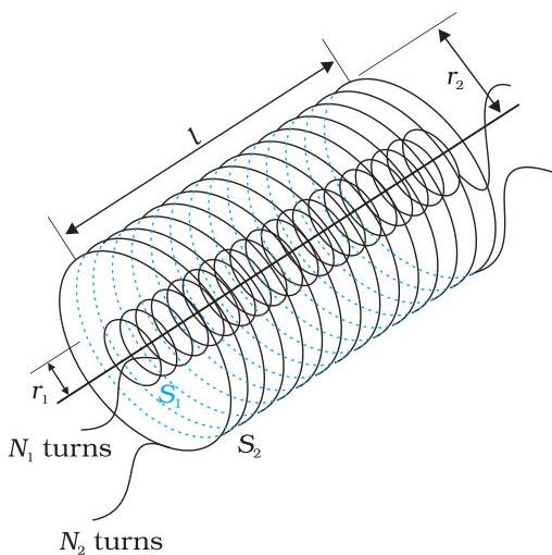 FIGURE 6.12 Two long co-axial solenoids of same length $l$.
Upon establishing a current $I_2$ within $S_2$, a magnetic flux is consequently generated through $S_1$. This flux is designated as $\Phi_1$. The resultant flux linkage with solenoid $S_1$ is given by:
$ N _ {1} \Phi_ {1} = M _ {1 2} I _ {2} \tag {6.7} $
$M_{12}$ represents the mutual inductance of solenoid $S_1$ relative to solenoid $S_2$, occasionally termed the coefficient of mutual induction.
The calculation of $M_{12}$ is feasible for this straightforward arrangement of co-axial solenoids. The magnetic field produced by current $I_2$ in $S_2$ is $\mu_0 n_2 I_2$. Consequently, the flux linkage with coil $S_1$ is:
$ \begin{array}{l} N _ {1} \Phi_ {1} = (n _ {1} l) (\pi r _ {1} ^ {2}) (\mu_ {0} n _ {2} I _ {2}) \ = \mu_ {0} n _ {1} n _ {2} \pi r _ {1} ^ {2} l I _ {2} \tag {6.8} \ \end{array} $
Here, $n_1l$ denotes the total turn count of solenoid $S_1$. Therefore, by comparing Eq. (6.7) and Eq. (6.8), we derive:
$ M _ {1 2} = \mu_ {0} n _ {1} n _ {2} \pi r _ {1} ^ {2} l \tag {6.9} $
It is important to acknowledge that edge effects were disregarded, and the magnetic field $\mu_0 n_2 I_2$ was assumed to be uniform across the entire length and cross-section of solenoid $S_2$. This constitutes a valid approximation, given the condition of a long solenoid, where $l \gg r_2$.
Shifting to the inverse scenario, if a current $I_1$ flows through solenoid $S_1$, the flux linkage with coil $S_2$ becomes:
$ N _ {2} \Phi_ {2} = M _ {2 1} I _ {1} \tag {6.10} $
$M_{21}$ designates the mutual inductance of solenoid $S_2$ relative to solenoid $S_1$.
Given the substantial length of the solenoids, the magnetic flux generated by current $I_1$ in $S_1$ may be considered to be entirely contained within $S_1$. Consequently, the flux linkage with solenoid $S_2$ is:
$ N _ {2} \Phi_ {2} = (n _ {2} l) (\pi r _ {1} ^ {2}) (\mu_ {0} n _ {1} I _ {1}) $
Here, $n_2l$ signifies the total turns of $\mathbf{S}_2$. Based on Eq. (6.10), we find:
$ M _ {2 1} = \mu_ {0} n _ {1} n _ {2} \pi r _ {1} ^ {2} l \tag {6.11} $
By comparing Eq. (6.9) and Eq. (6.10), it is evident that:
$ M _ {1 2} = M _ {2 1} = M (\text {say}) \tag {6.12} $
While this equivalence has been established for the specific case of long co-axial solenoids, the principle itself possesses broader applicability. Consider, for instance, a situation where the inner solenoid is significantly shorter than and positioned centrally within the outer solenoid. In such a configuration, determining the flux linkage $N_1\Phi_1$ remains straightforward, as the inner solenoid is effectively bathed in a uniform magnetic field originating from the outer solenoid. Under these conditions, the computation of $M_{12}$ would be relatively simple. Conversely, calculating the flux linkage with the outer solenoid would present considerable difficulty, owing to the non-uniformity of the magnetic field produced by the inner solenoid across both the length and cross-section of the outer coil. Thus, the determination of $M_{21}$ would be exceptionally challenging in this particular scenario. The established equality $M_{12} = M_{21}$ proves immensely valuable in resolving such complex situations.
Electromagnetic Induction
In the preceding discussion, the medium within the solenoids was assumed to be air. However, if a material possessing a relative permeability of $\mu_r$ were introduced, the mutual inductance would then be given by:
$ M = \mu_r \mu_0 n_1 n_2 \pi r_1^2 I $
Furthermore, it is crucial to recognize that the mutual inductance between components such as coils or solenoids is contingent upon both their spatial separation and their relative angular alignment.
Example 6.8 Consider two concentric circular coils, positioned co-axially with their centers aligned. One coil has a small radius, $r_1$, while the other possesses a significantly larger radius, $r_2$, satisfying the condition $r_1 \ll r_2$. Determine the mutual inductance for this configuration.
Solution If a current $I_2$ traverses the larger circular coil, the magnetic field strength at its center is given by $B_2 = \mu_0 I_2 / (2r_2)$. Given that the inner co-axial coil has a considerably smaller radius, the magnetic field $B_2$ can be approximated as uniform across its entire cross-sectional area. Consequently,
$ \begin{array}{l} \Phi_ {1} = \pi r _ {1} ^ {2} B _ {2} \ = \frac {\mu_ {0} \pi r _ {1} ^ {2}}{2 r _ {2}} I _ {2} \ = M _ {1 2} I _ {2} \ \end{array} $
Thus,
$ M _ {1 2} = \frac {\mu_ {0} \pi r _ {1} ^ {2}}{2 r _ {2}} $
From Eq. (6.12)
$ M _ {1 2} = M _ {2 1} = \frac {\mu_ {0} \pi r _ {1} ^ {2}}{2 r _ {2}} $
It should be noted that the calculation of $M_{12}$ relies on an approximation of $\Phi_1$, specifically by presuming the magnetic field $B_2$ to be spatially uniform across the area $\pi r_1^2$. This approximation is justifiable and acceptable due to the condition $r_1 \ll r_2$.
Recalling Experiment 6.3 from Section 6.2, an electromotive force (emf) was observed to be induced in coil $C_1$ whenever the current flowing through coil $C_2$ underwent a change. If $\Phi_1$ represents the magnetic flux linkage through coil $C_1$ (which possesses $N_1$ turns) when a current $I_2$ is present in coil $C_2$,
Then, consistent with Equation (6.7), it follows that:
$ N _ {1} \Phi_ {1} = M I _ {2} $
When considering time-varying currents,
$ \frac {\mathrm {d} \left(N _ {1} \Phi_ {1}\right)}{\mathrm {d} t} = \frac {\mathrm {d} \left(M I _ {2}\right)}{\mathrm {d} t} $
Given that the induced electromotive force in coil $C_1$ is defined as:
$ \varepsilon_ {1} = - \frac {\mathrm {d} \left(N _ {1} \Phi_ {1}\right)}{\mathrm {d} t} $
We get,
$ \varepsilon_ {1} = - M \frac {\mathrm {d} I _ {2}}{\mathrm {d} t} $
This relationship demonstrates that a time-varying current within one coil is capable of inducing an electromotive force in an adjacent coil. The amplitude of this induced emf is directly proportional to both the rate of change of current and the mutual inductance between the two coils.
6.7.2 Self-inductance
While the preceding section focused on the magnetic flux generated in one solenoid by the current flowing through another, it is equally possible for an electromotive force (emf) to be induced within an individual, isolated coil. This occurs when the magnetic flux passing through the coil changes due to variations in the current within that very coil. This phenomenon is termed self-induction. In such instances, the total magnetic flux linkage, encompassing $N$ turns of the coil, is directly proportional to the current traversing the coil, represented as:
$ N \Phi_{B} \propto I $
$ N \Phi_{B} = L I \tag{6.13} $
Here, the proportionality constant, $L$, is designated as the self-inductance of the coil, sometimes also referred to as the coefficient of self-induction. When the current is altered, the magnetic flux linked with the coil consequently changes, leading to the induction of an emf within the coil. Based on Equation (6.13), the induced emf can be expressed as:
$ \varepsilon = - \frac {\mathrm {d} (N \Phi_{B})}{\mathrm {d} t} $
$ \varepsilon = - L \frac {\mathrm {d} I}{\mathrm {d} t} \tag{6.14} $
Consequently, the self-induced emf consistently acts to counteract any modification (whether an increase or decrease) in the current flowing through the coil.
The self-inductance can be computed for circuits exhibiting straightforward geometric configurations. Consider, for example, a long solenoid with a cross-sectional area $A$ and length $l$, possessing $n$ turns per unit length. The magnetic field produced by a current $I$ passing through this solenoid is given by $B = \mu_0 n I$ (assuming negligible edge effects, as in previous analyses). The total magnetic flux linked with the solenoid is therefore:
$ \begin{array}{l} N \Phi_{B} = (n l) (\mu_{0} n I) (A) \ = \mu_{0} n^{2} A l I \ \end{array} $
where $nl$ represents the cumulative number of turns. Thus, the self-inductance is determined by:
$ \begin{array}{l} L = \frac {N \Phi_{B}}{I} \ = \mu_{0} n^{2} A l \tag{6.15} \ \end{array} $
Should the interior of the solenoid be filled with a material characterized by a relative permeability $\mu_r$ (such as soft iron, which possesses a high relative permeability value), the self-inductance then becomes:
$ L = \mu_{r} \mu_{0} n^{2} A l \tag{6.16} $
It is evident that the self-inductance of a coil is contingent upon its physical geometry and the magnetic permeability of the surrounding medium.
The self-induced emf is also commonly termed a back emf because its direction consistently opposes any alteration in the current within a circuit. From a physical perspective, self-inductance
functions analogously to inertia. It serves as the electromagnetic counterpart to mass in mechanical systems. Therefore, energy must be expended to overcome this back emf $(\varepsilon)$ when establishing a current. This expended energy is subsequently stored as magnetic potential energy. For a current $I$ present in a circuit at a given instant, the rate at which work is performed is:
$ \frac {\mathrm {d} W}{\mathrm {d} t} = | \varepsilon | I $
If resistive losses are disregarded, and only the inductive effect is considered, then by utilizing Equation (6.14), we find:
$ \frac {\mathrm {d} W}{\mathrm {d} t} = L I \frac {\mathrm {d} I}{\mathrm {d} t} $
The cumulative work done to establish the current $I$ is obtained by integrating this expression:
$ W = \int \mathrm {d} W = \int_ {0} ^ {I} L I \mathrm {d} I $
Hence, the energy required to build up the current to a value $I$ is:
$ W = \frac {1}{2} L I ^ {2} \tag {6.17} $
This formula bears a striking resemblance to $m v^{2} / 2$, which represents the (mechanical) kinetic energy of a particle with mass $m$. This parallel underscores that $L$ is analogous to $m$, signifying that $L$ represents electrical inertia, which resists both the increase and decrease of current in the circuit.
When considering the general scenario where currents flow simultaneously within two closely positioned coils, the magnetic flux linked with one coil will constitute the sum of two independently existing flux components. This necessitates a modification of the flux linkage equation, yielding:
$ N _ {1} \Phi_ {1} = M _ {1 1} I _ {1} + M _ {1 2} I _ {2} $
Here, $M_{11}$ denotes the inductance attributed to the coil itself.
Consequently, by applying Faraday's law of electromagnetic induction, we obtain:
$ \varepsilon_ {1} = - M _ {1 1} \frac {\mathrm {d} I _ {1}}{\mathrm {d} t} - M _ {1 2} \frac {\mathrm {d} I _ {2}}{\mathrm {d} t} $
The term $M_{11}$ is identified as the self-inductance and is conventionally represented as $L_1$. Therefore, the expression becomes:
$ \varepsilon_ {1} = - L _ {1} \frac {\mathrm {d} I _ {1}}{\mathrm {d} t} - M _ {1 2} \frac {\mathrm {d} I _ {2}}{\mathrm {d} t} $
Example 6.9 (a) Obtain the expression for the magnetic energy stored in a solenoid in terms of magnetic field $B$, area $A$ and length $l$ of the solenoid. (b) How does this magnetic energy compare with the electrostatic energy stored in a capacitor?
Solution
(a) From Equation (6.17), the magnetic energy is determined as:
$ \begin{array}{l} U _ {B} = \frac {1}{2} L I ^ {2} \ = \frac {1}{2} L \left(\frac {B}{\mu_ {0} n}\right) ^ {2} \quad \left(\text {since} B = \mu_ {0} n I, \text {for a solenoid}\right) \ \end{array} $
$
\begin{array}{l} = \frac {1}{2} \left(\mu_ {0} n ^ {2} A l\right) \left(\frac {B}{\mu_ {0} n}\right) ^ {2} \quad [ \text {from Eq. (6.15)} ] \ = \frac {1}{2 \mu_ {0}} B ^ {2} A l \ \end{array} $
(b) The magnetic energy normalized by volume is given by:
$ \begin{array}{l} u _ {B} = \frac {U _ {B}}{V} \quad (\text {where } V \text { is volume that contains flux}) \ = \frac {U _ {B}}{A l} \ = \frac {B ^ {2}}{2 \mu_ {0}} \tag {6.18} \ \end{array} $
The relationship for the electrostatic energy stored per unit volume within a parallel plate capacitor has previously been established (refer to Chapter 2, Equation 2.73):
$ u _ {E} = \frac {1}{2} \varepsilon_ {0} E ^ {2} \tag {2.73} $
In both instances, the energy is directly proportional to the square of the respective field strength. While Equations (6.18) and (2.73) were derived from specific configurations—a solenoid and a parallel plate capacitor, respectively—their applicability is universal, extending to any spatial domain where a magnetic field and/or an electric field is present.
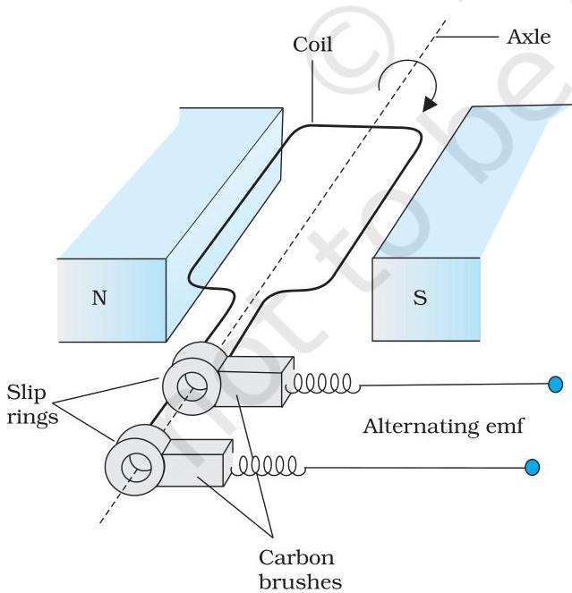 FIGURE 6.13 AC Generator
6.8 AC GENERATOR
The principle of electromagnetic induction finds numerous technological applications, with a particularly significant one being the generation of alternating currents (AC). Contemporary AC generators, often featuring output capacities around $100\mathrm{MW}$, represent sophisticated engineering. This section will elucidate the fundamental operational concepts of such devices, whose development is frequently attributed to the Yugoslav innovator, Nicola Tesla. As previously established in Section 6.3, an electromotive force (EMF) or current can be induced in a conductive loop by altering its orientation or its effective area. When a coil rotates within a magnetic field $\mathbf{B}$, the effective area of the loop — defined as the surface perpendicular to the field lines — is given by $A \cos \theta$, where $\theta$ signifies the angle between the area vector $\mathbf{A}$ and the magnetic field vector $\mathbf{B}$. This mechanism of varying magnetic flux constitutes the core principle governing a basic
AC generator, which functions by transforming mechanical energy into electrical energy.
Figure 6.13 illustrates the fundamental components of an AC generator. The apparatus primarily comprises a coil affixed to a rotor shaft, engineered such that the coil's rotational axis is orthogonal to the magnetic field's orientation. This coil, also known as the armature, is mechanically actuated by an external power source to rotate within the uniform magnetic field. This rotation inherently modifies the magnetic flux traversing the coil, thereby inducing an electromotive force within it. Electrical connectivity between the coil terminals and an external circuit is established through a system of slip rings and brushes.
Upon rotating the coil at a uniform angular velocity $\omega$, the instantaneous angle $\theta$ between the magnetic field vector $\mathbf{B}$ and the coil's area vector $\mathbf{A}$ at time $t$ is given by $\theta = \omega t$ (presuming an initial condition of $\theta = 0^{\circ}$ at $t = 0$). Consequently, the portion of the coil's effective area interacting with the magnetic field lines undergoes continuous variation over time. Drawing from Equation (6.1), the magnetic flux at any given instant $t$ is expressed as:
$ \phi_{\mathrm{B}} = BA \cos \theta = BA \cos \omega t $
According to Faraday's law of electromagnetic induction, the electromotive force induced in a rotating coil comprising $N$ turns is subsequently calculated as:
$ \varepsilon = -N \frac{\mathrm{d} \phi_{\mathrm{B}}}{\mathrm{d} t} = -NBA \frac{\mathrm{d}}{\mathrm{d} t} (\cos \omega t) $
Therefore, the instantaneous magnitude of the induced electromotive force is:
$ \varepsilon = NBA \omega \sin \omega t \tag{6.19} $
Here, $NBA\omega$ represents the peak electromotive force, which is realized when the term $\sin \omega t$ equals $\pm 1$. Should we designate $NBA\omega$ as $\varepsilon_0$, the expression then becomes:
$ \varepsilon = \varepsilon_0 \sin \omega t \tag{6.20} $
Given that the sine function's range spans from $+1$ to $-1$, the polarity of the induced electromotive force inherently oscillates over time. As depicted in Fig. 6.14, the EMF attains its maximum or minimum (extremum) values when $\theta = 90^{\circ}$ or $\theta = 270^{\circ}$, a consequence of the magnetic flux undergoing its most significant rate of change at these specific orientations.
The current's direction undergoes periodic reversal, which is why it is termed an alternating current (AC). Recognizing that $\omega = 2\pi \nu$, Equation (6.20) may alternatively be expressed as:
$ \varepsilon = \varepsilon_0 \sin 2\pi \nu t \tag{6.21} $
Here, $\nu$ represents the rotational frequency of the generator's coil.
It is important to recognize that Equations (6.20) and (6.21) express the instantaneous electromotive force (emf), with $\varepsilon$ oscillating periodically between its peak positive value of $+\varepsilon_0$ and peak negative value of $-\varepsilon_0$. The methodology for calculating the time-averaged magnitude of alternating voltage and current will be explored in the subsequent chapter.
Commercial power generation relies on various sources to provide the mechanical energy needed to rotate the armature. For instance, water descending from significant elevations, such as from dams, powers hydro-electric generators. Another common approach involves heating water to generate high-pressure steam, often using coal or other fuel sources, which then drives the armature's rotation; these are known as thermal generators. Should nuclear fuel be employed instead of coal, the result is a nuclear power generator. Contemporary generators are capable of producing substantial electrical power, reaching outputs of up to 500 MW, which is sufficient to illuminate five million $100\mathrm{W}$ bulbs.
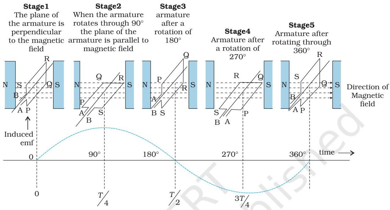 FIGURE 6.14 An alternating emf is generated by a loop of wire rotating in a magnetic field.
It is noteworthy that in the majority of modern generators, the coils remain static, while the electromagnets are the rotating components. The standard operational frequency for rotation is $50\mathrm{Hz}$ in India, whereas in some nations, like the USA, it is $60\mathrm{Hz}$.
Example 6.10
Kamla peddles a stationary bicycle. The pedals of the bicycle are attached to a 100 turn coil of area $0.10\mathrm{m}^2$. The coil rotates at half a revolution per second and it is placed in a uniform magnetic field of $0.01\mathrm{T}$ perpendicular to the axis of rotation of the coil. What is the maximum voltage generated in the coil?
Solution Here $\nu = 0.5\mathrm{Hz}$ ; $N = 100$ , $A = 0.1\mathrm{m}^2$ and $B = 0.01\mathrm{T}$ . Employing Eq. (6.19)
$ \begin{array}{l} \varepsilon_ {0} = N B A (2 \pi v) \ = 1 0 0 \times 0. 0 1 \times 0. 1 \times 2 \times 3. 1 4 \times 0. 5 \ = 0. 3 1 4 \mathrm {V} \ \end{array} $
The maximum voltage is $0.314\mathrm{V}$
We urge you to explore such alternative possibilities for power generation.
SUMMARY
- The magnetic flux through a surface of area $\mathbf{A}$ placed in a uniform magnetic field $\mathbf{B}$ is defined as,
$ \Phi_{\mathrm{B}} = \mathbf{B} \cdot \mathbf{A} = B A \cos \theta $
where $\theta$ is the angle between $\mathbf{B}$ and $\mathbf{A}$.
- Faraday's laws of induction imply that the emf induced in a coil of $N$ turns is directly related to the rate of change of flux through it,
$ \varepsilon = - N \frac {\mathrm {d} \Phi_ {\mathrm {B}}}{\mathrm {d} t} $
Here $\Phi_{\mathrm{B}}$ is the flux linked with one turn of the coil. If the circuit is closed, a current $I = \varepsilon / R$ is set up in it, where $R$ is the resistance of the circuit.
Lenz's law states that the polarity of the induced emf is such that it tends to produce a current which opposes the change in magnetic flux that produces it. The negative sign in the expression for Faraday's law indicates this fact.
When a metal rod of length $l$ is placed normal to a uniform magnetic field $B$ and moved with a velocity $v$ perpendicular to the field, the induced emf (called motional emf) across its ends is
$ \varepsilon = B l v $
Inductance is the ratio of the flux-linkage to current. It is equal to $N\Phi / l$.
A changing current in a coil (coil 2) can induce an emf in a nearby coil (coil 1). This relation is given by,
$ \varepsilon_ {1} = - M _ {1 2} \frac {\mathrm {d} I _ {2}}{\mathrm {d} t} $
The quantity $M_{12}$ is called mutual inductance of coil 1 with respect to coil 2. One can similarly define $M_{21}$. There exists a general equality,
$ M _ {1 2} = M _ {2 1} $
- When a current in a coil changes, it induces a back emf in the same coil. The self-induced emf is given by,
$ \varepsilon = - L \frac {\mathrm {d} I}{\mathrm {d} t} $
$L$ is the self-inductance of the coil. It is a measure of the inertia of the coil against the change of current through it.
- The self-inductance of a long solenoid, the core of which consists of a magnetic material of relative permeability $\mu_{\mathrm{r}}$, is given by
$ L = \mu_ {r} \mu_ {0} n ^ {2} A l $
where $A$ is the area of cross-section of the solenoid, $l$ its length and $n$ the number of turns per unit length.
- In an ac generator, mechanical energy is converted to electrical energy by virtue of electromagnetic induction. If coil of $N$ turn and area $A$ is rotated at $\nu$ revolutions per second in a uniform magnetic field $B$, then the motional emf produced is
$ \varepsilon = N B A (2 \pi \nu) \sin (2 \pi \nu t) $
where we have assumed that at time $t = 0$ s, the coil is perpendicular to the field.
| Quantity | Symbol | Units | Dimensions | Equations |
|---|---|---|---|---|
| Magnetic Flux | $\Phi_{\mathrm{B}}$ | Wb (weber) | [M L$^{2}$ T$^{-2}$ A$^{-1}$] | $\Phi_{\mathrm{B}}$ = $\mathbf{B} \cdot \mathbf{A}$ |
| EMF | $\varepsilon$ | V (volt) | [M L$^{2}$ T$^{-3}$ A$^{-1}$] | $\varepsilon$ = -d(N$\Phi_{\mathrm{B}}$)/dt |
| Mutual Inductance | M | H (henry) | [M L$^{2}$ T$^{-2}$ A$^{-2}$] | $\varepsilon_{1}$ = -M${12}$(dI${2}$/dt) |
| Self Inductance | L | H (henry) | [M L$^{2}$ T$^{-2}$ A$^{-2}$] | $\varepsilon$ = -L(dI/dt) |
POINTS TO PONDER
- Electricity and magnetism are intimately related. In the early part of the nineteenth century, the experiments of Oersted, Ampere and others established that moving charges (currents) produce a magnetic field. Somewhat later, around 1830, the experiments of Faraday and Henry demonstrated that a moving magnet can induce electric current.
- In a closed circuit, electric currents are induced so as to oppose the changing magnetic flux. It is as per the law of conservation of energy. However, in case of an open circuit, an emf is induced across its ends. How is it related to the flux change?
- The motional emf discussed in Section 6.5 can be argued independently from Faraday's law using the Lorentz force on moving charges. However, even if the charges are stationary [and the $q(\mathbf{v} \times \mathbf{B})$ term of the Lorentz force is not operative], an emf is nevertheless induced in the presence of a time-varying magnetic field. Thus, moving charges in static field and static charges in a time-varying field seem to be symmetric situation for Faraday's law. This gives a tantalising hint on the relevance of the principle of relativity for Faraday's law.
EXERCISES
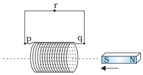
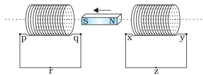
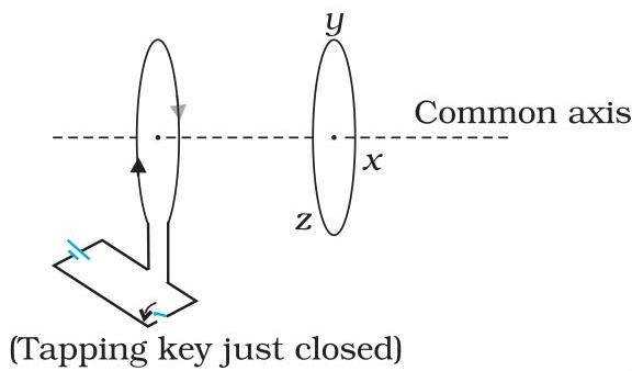
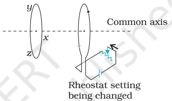
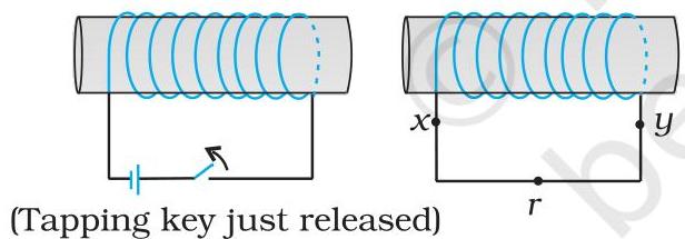
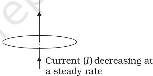
6.1 For the scenarios illustrated in Figures 6.15(a) through (f), ascertain the direction of the induced electric current.
 (a)
(a)
 (b)
(b)
 (c)
(c)
 (d)
(d)
 (e)
FIGURE 6.15
(e)
FIGURE 6.15
 (f)
(f)
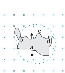
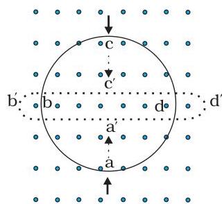
6.2 Apply Lenz's principle to establish the orientation of the induced electrical current within the contexts presented in Figure 6.16:
(a) An irregularly shaped conductor undergoing transformation into a circular configuration;
(b) A circular conductive loop undergoing deformation into a slender linear conductor.
 (a)
(a)
 (b)
FIGURE 6.16
(b)
FIGURE 6.16
6.3 Consider a lengthy solenoid possessing a turn density of 15 turns per centimeter, within which a compact loop, with an area of $2.0\mathrm{cm}^2$, is positioned perpendicularly to the solenoid's central axis. Should the current traversing the solenoid undergo a uniform alteration from 2.0 A to 4.0 A over a duration of 0.1 seconds, what electromotive force (emf) is induced in the loop during this period of current variation?
6.4 A rectangular wire loop, measuring $8\mathrm{cm}$ by $2\mathrm{cm}$ and featuring a narrow incision, is being withdrawn from an area permeated by a uniform magnetic field of $0.3\mathrm{T}$, with the field lines oriented perpendicularly to the loop's plane. Determine the electromotive force generated across the incision if the loop's translational speed is $1\mathrm{cm}\mathrm{s}^{-1}$, with its motion perpendicular to (a) its longer dimension, and (b) its shorter dimension. In each scenario, what is the duration for which the induced potential difference persists?
6.5 A metallic rod, $1.0\mathrm{m}$ in length, undergoes rotation at an angular frequency of $400\mathrm{rads^{-1}}$ around an axis that is perpendicular to the rod and passes through one of its extremities. The opposing end of the rod maintains contact with a concentric metallic ring. A magnetic field, uniform and constant with a magnitude of $0.5\mathrm{T}$, is present throughout the region, oriented parallel to the axis of rotation. Compute the electromotive force induced between the rotational pivot and the metallic ring.
6.6 A straight horizontal conductor, $10\mathrm{m}$ in length and oriented from east to west, is descending at a velocity of $5.0\mathrm{ms^{-1}}$. This motion occurs perpendicularly to the horizontal component of Earth's magnetic field, which has a magnitude of $0.30 \times 10^{-4}\mathrm{Wb~m}^{-2}$.
(a) Determine the instantaneous magnitude of the electromotive force generated within the conductor. (b) Specify the polarity of the induced electromotive force. (c) Identify which extremity of the conductor possesses the greater electrical potential.
6.7 The electrical current within a circuit decreases from 5.0 A to 0.0 A over a time interval of 0.1 seconds. Given that an average electromotive force of $200\mathrm{V}$ is induced, provide an approximation for the circuit's self-inductance. 6.8 Two proximate coils exhibit a mutual inductance of $1.5\mathrm{H}$. Should the current flowing through one of these coils vary from 0 to $20\mathrm{A}$ within $0.5\mathrm{s}$, what is the corresponding alteration in magnetic flux linkage experienced by the second coil?