ELECTROSTATIC POTENTIAL AND CAPACITANCE - CBSE Class 12 Physics Notes

Chapter Two

ELECTROSTATIC POTENTIAL AND CAPACITANCE

2.1 INTRODUCTION

The concept of potential energy was previously established in Chapters 5 and 7 (Class XI). When an external agency performs work to displace an object from one location to another, counteracting a force such as a spring force or gravitational force, this work is accumulated as the object's potential energy. Upon the cessation of the external force, the object undergoes motion, converting an equivalent quantity of potential energy into kinetic energy. Consequently, the total sum of kinetic and potential energies remains constant. Forces exhibiting this characteristic are designated as conservative forces, with spring force and gravitational force serving as archetypal instances.

Similarly, the Coulombic force between two static charges is also a conservative force. This similarity is expected, given that both the gravitational and Coulombic forces exhibit an inverse-square relationship with distance, primarily differing in their proportionality constants; specifically, charges substitute for masses in the context of Coulomb's law compared to the gravitational law. Therefore, analogous to the potential energy of a mass within a gravitational field, we can establish the electrostatic potential energy for a charge situated in an electrostatic field.

Let us consider an electrostatic field $\mathbf{E}$ originating from a particular charge arrangement. Initially, for ease of comprehension, we will focus on the field $\mathbf{E}$ generated by a charge $Q$ positioned at the origin. Now, envision the process of transporting a test charge $q$ from point $R$ to point $P$, necessitating work against the repulsive force exerted upon it by charge $Q$. In conjunction

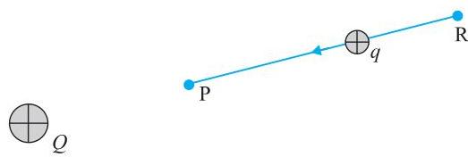FIGURE 2.1 A test charge $q (>0)$ is moved from the point R to the point P against the repulsive force on it by the charge $Q (>0)$ placed at the origin.

with Fig. 2.1, this scenario occurs if both $Q$ and $q$ possess either positive or negative charges. For the purpose of clear illustration, we shall assume that both $Q$ and $q$ are greater than zero.

Two important considerations are pertinent at this juncture. Firstly, it is presupposed that the test charge $q$ is of sufficiently negligible magnitude that it does not perturb the initial charge configuration, specifically the charge $Q$ situated at the origin (alternatively, $Q$ is maintained in its fixed position at the origin by an unspecified force). Secondly, during the transit of charge $q$ from R to P, an external force $\mathbf{F}{\mathrm{ext}}$ is applied, precisely balancing the repulsive electric force $\mathbf{F}{\mathrm{E}}$ (i.e., $\mathbf{F}{\mathrm{ext}} = -\mathbf{F}{\mathrm{E}}$). This implies that the charge $q$ experiences no net force or acceleration as it is moved from R to P, signifying its transport at an infinitesimally slow, constant velocity. Under

these circumstances, the work performed by the external force is equivalent to the negative of the work exerted by the electric force, and this work is entirely converted into the potential energy of the charge $q$. Should the external force be withdrawn upon reaching point P, the electric force will propel the charge away from Q; the potential energy accumulated at P is then utilized to impart kinetic energy to charge $q$, ensuring that the aggregate of kinetic and potential energies remains invariant.

Consequently, the work executed by external forces in displacing a charge $q$ from R to P is

$ \begin{array}{l} \mathrm {W} _ {\mathrm {R P}} = \int_ {\mathrm {R}} ^ {\mathrm {P}} \mathbf {F} _ {\text {e x t}} \cdot \mathrm {d} \mathbf {r} \ = - \int_ {\mathrm {R}} ^ {\mathrm {P}} \mathbf {F} _ {\text {e x t}} \cdot \mathrm {d} \mathbf {r} \tag {2.1} \ \end{array} $ The effort expended here counters the electrostatic repulsive force, manifesting as stored potential energy.

Within an electric field, a charged particle ($q$) inherently holds a specific electrostatic potential energy. The work performed, as described, augments this potential energy by an increment precisely equivalent to the potential energy differential between points R and P.

Consequently, the potential energy difference is expressed as:

$ \Delta U = U _ {P} - \bar {U} _ {R} = W _ {R P} \tag {2.2} $

(It should be noted that this displacement occurs in a direction contrary to the electric force, implying that the work performed by the electric field is negative, specifically $-W_{RP}$.)

Accordingly, the electric potential energy difference between any two points may be characterized as the work an external force must exert to transport a charge $q$ from one point to the other (without inducing acceleration) within the electric field generated by an arbitrary charge arrangement.

Two crucial observations can be presented at this juncture:

(i) The expression on the right-hand side of Equation (2.2) is solely determined by the charge's initial and terminal positions. This signifies that the work executed by an electrostatic field in displacing a charge between two points is contingent exclusively upon these start and end points, showing no dependence on the trajectory followed. This property is a defining feature of a conservative force. The utility of the potential energy concept would be diminished if the work were path-dependent. The independence of path for work performed by an electrostatic field can be demonstrated via Coulomb's law; however, this derivation is omitted for brevity.

(ii) Equation (2.2) establishes the potential energy difference using work, a quantity with physical significance. Evidently, potential energy, as defined in this manner, possesses an inherent ambiguity up to an arbitrary additive constant. This implies that the absolute magnitude of potential lacks physical importance; rather, it is solely the difference in potential energy that holds physical meaning. An arbitrary constant $\alpha$ can invariably be appended to the potential energy at every location without altering the potential energy difference, as shown:

$ (U_p + \alpha) - (U_R + \alpha) = U_p - U_R $

Alternatively, flexibility exists in designating the reference point where potential energy is zero. A practical convention involves setting the electrostatic potential energy to zero at infinity. Adopting this convention, if we consider point R to be at infinity, Equation (2.2) yields:

$ W_{\infty P} = U_p - U_{\infty} = U_P \tag{2.3} $

As point P is arbitrary, Equation (2.3) furnishes a definition for the potential energy of a charge $q$ at any given location. Specifically, the potential energy of charge $q$ at a particular point (within the field established by any charge configuration) is equivalent to the work performed by an external force (which is equal in magnitude and opposite in direction to the electric force) to transport the charge $q$ from infinity to that designated point.

2.2 ELECTROSTATIC POTENTIAL

For any general static charge configuration, the potential energy of a test charge $q$ is defined in relation to the work exerted upon it. This work is inherently proportional to $q$, as the force experienced at any point is $q\mathbf{E}$, where $\mathbf{E}$ denotes the electric field at that location due to the specified charge configuration. Therefore, it is advantageous to normalize the work by dividing it by the charge $q$, yielding a quantity independent of $q$. Essentially, the work done per unit test charge is a characteristic attribute of the electric field associated with the charge configuration. This foundational idea introduces the concept of electrostatic potential $V$ for a particular charge arrangement. Referring to Eq. (2.1), we obtain:

The work performed by an external force to transport a unit positive charge from point R to P is expressed as:

$ = V_P - V_R \left(= \frac{U_P - U_R}{q}\right) \tag{2.4} $

Here, $V_P$ and $V_R$ designate the electrostatic potentials at points P and R, respectively. It is crucial to recall, consistent with previous discussions, that the absolute magnitude of potential lacks physical significance; rather, it is the potential difference that holds physical meaning. Should we, as previously established, define the potential at infinity as zero, then Eq. (2.4) consequently signifies:

The work performed by an external force to move a unit positive charge from an infinite distance to a specific point defines the electrostatic potential ($V$) at that point.

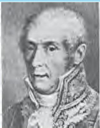
Count Alessandro Volta (1745 - 1827) was an Italian physicist and a professor at Pavia. Volta demonstrated that the phenomenon of animal electricity, which Luigi Galvani (1737-1798) had observed during experiments involving frog muscle tissue in contact with disparate metals, did not originate from unique characteristics of animal tissues. Instead, he proved that such electrical generation occurred universally whenever a moistened substance was positioned between two different metals. This pivotal discovery prompted his invention of the initial voltaic pile, or battery, which comprised multiple layers of damp cardboard disks (acting as the electrolyte) interleaved with metallic disks (serving as electrodes).

Physics

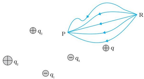FIGURE 2.2 Work done on a test charge $q$ by the electrostatic field due to any given charge configuration is independent of the path, and depends only on its initial and final positions.

In other words, the electrostatic potential $(V)$ at any point in a region with electrostatic field is the work done in bringing a unit positive charge (without acceleration) from infinity to that point.

The qualifying remarks made earlier regarding potential energy also apply to the definition of potential. To obtain the work done per unit test charge, we should take an infinitesimal test charge $\delta q$, obtain the work done $\delta W$ in bringing it from infinity to the point and determine the ratio $\delta W / \delta q$. Also, the external force at every point of the path is to be equal and opposite to the electrostatic force on the test charge at that point.

2.3 POTENTIAL DUE TO A POINT CHARGE

Consider a point charge $Q$ at the origin (Fig. 2.3). For definiteness, take $Q$ to be positive. We wish to determine the potential at any point $P$ with

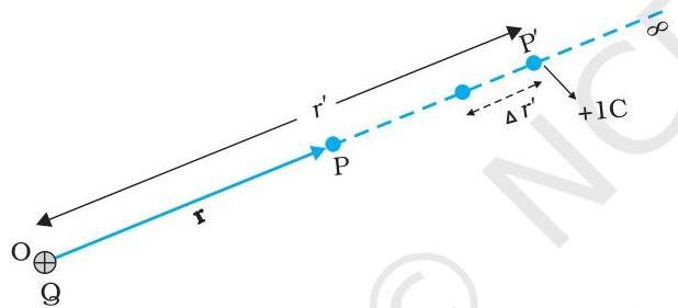FIGURE 2.3 Work done in bringing a unit positive test charge from infinity to the point P, against the repulsive force of charge $Q$ ($Q > 0$), is the potential at P due to the charge $Q$.

position vector $\mathbf{r}$ from the origin. For that we must calculate the work done in bringing a unit positive test charge from infinity to the point P. For $Q > 0$, the work done against the repulsive force on the test charge is positive. Since work done is independent of the path, we choose a convenient path - along the radial direction from infinity to the point P.

At some intermediate point $\mathbf{P}'$ on the path, the electrostatic force on a unit positive charge is

$ \frac {Q \times 1}{4 \pi \varepsilon_ {0} r ^ {\prime 2}} \hat {\mathbf {r}} ^ {\prime} \tag {2.5} $

where $\hat{\mathbf{r}}'$ is the unit vector along $\mathrm{OP}'$. Work done against this force from $\mathbf{r}'$ to $\mathbf{r}' + \Delta \mathbf{r}'$ is

$ \Delta W = - \frac {Q}{4 \pi \varepsilon_ {0} r ^ {\prime 2}} \Delta r ^ {\prime} \tag {2.6} $

The negative sign appears because for $\Delta r' < 0$, $\Delta W$ is positive. Total work done (W) by the external force is obtained by integrating Eq. (2.6) from $r' = \infty$ to $r' = r$,

$ W = - \int_ {\infty} ^ {r} \frac {Q}{4 \pi \varepsilon_ {0} r ^ {\prime 2}} d r ^ {\prime} = \frac {Q}{4 \pi \varepsilon_ {0} r ^ {\prime}} \Bigg | _ {\infty} ^ {r} = \frac {Q}{4 \pi \varepsilon_ {0} r} \tag {2.7} $

This, by definition is the potential at $\mathbf{P}$ due to the charge $Q$

$ V (r) = \frac {Q}{4 \pi \varepsilon_ {0} r} \tag {2.8} $

Equation (2.8) is true for any sign of the charge $Q$, though we considered $Q > 0$ in its derivation. For $Q < 0$, $V < 0$, i.e., work done (by the external force) per unit positive test charge in bringing it from infinity to the point is negative. This is equivalent to saying that work done by the electrostatic force in bringing the unit positive charge form infinity to the point $P$ is positive. [This is as it should be, since for $Q < 0$, the force on a unit positive test charge is attractive, so that the electrostatic force and the displacement (from infinity to $P$) are in the same direction.] Finally, we note that Eq. (2.8) is consistent with the choice that potential at infinity be zero.

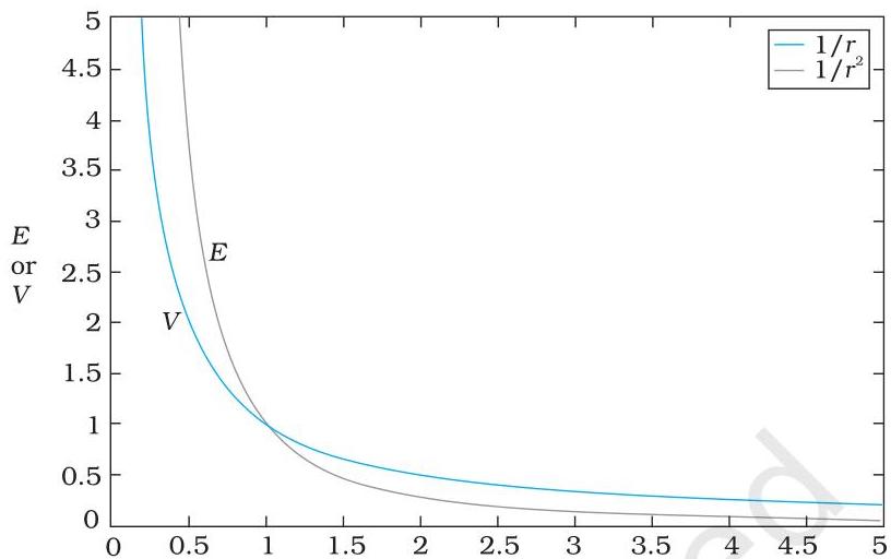FIGURE 2.4 Variation of potential $V$ with $r$ [in units of $(Q / 4\pi \varepsilon_0)\mathrm{m}^{-1}]$ (blue curve) and field with $r$ [in units of $(Q / 4\pi \varepsilon_0)\mathrm{m}^{-2}]$ (black curve) for a point charge $Q$.

Figure (2.4) shows how the electrostatic potential $(\propto 1 / r)$ and the electrostatic field $(\propto 1 / r^2)$ varies with $r$.

Example 2.1

(a) Calculate the potential at a point $P$ due to a charge of $4 \times 10^{-7} C$ located 9 cm away. (b) Hence obtain the work done in bringing a charge of $2 \times 10^{-9} \mathrm{C}$ from infinity to the point $P$. Does the answer depend on the path along which the charge is brought?

Solution

(a) $V = \frac{1}{4\pi\varepsilon_0}\frac{Q}{r} = 9\times 10^9\mathrm{Nm}^2\mathrm{C}^{-2}\times \frac{4\times 10^{-7}\mathrm{C}}{0.09\mathrm{m}}$ $= 4\times 10^{4}\mathrm{V}$ (b) $W = qV = 2 \times 10^{-9} \mathrm{C} \times 4 \times 10^{4} \mathrm{V}$ $= 8 \times 10^{-5} \mathrm{J}$

No, the work done is path-independent. Any infinitesimal segment of a path can be decomposed into two perpendicular components: one parallel to $\mathbf{r}$ and the other orthogonal to $\mathbf{r}$. The work contribution from the component orthogonal to $\mathbf{r}$ is zero.

2.4 POTENTIAL DUE TO AN ELECTRIC DIPOLE

Recalling our previous discussions, an electric dipole comprises two charges, $q$ and $-q$, separated by a minor distance, denoted $2\alpha$. The net charge of this configuration is zero. A dipole is defined by its dipole moment vector, $\mathbf{p}$, which has a magnitude of $q \times 2\alpha$ and is oriented from the negative charge to the positive charge (refer to Fig. 2.5). We previously observed that the electric field generated by a dipole at a location specified by position vector $\mathbf{r}$ is contingent not merely on the radial distance $r$, but also on the angular relationship between $\mathbf{r}$ and $\mathbf{p}$. Moreover, at considerable distances, the field strength diminishes proportionally to $1/r^3$, rather than the $1/r^2$ dependence characteristic of a single point charge. Our current objective is to ascertain the electric potential arising from a dipole and to draw comparisons with the potential produced by an isolated charge.

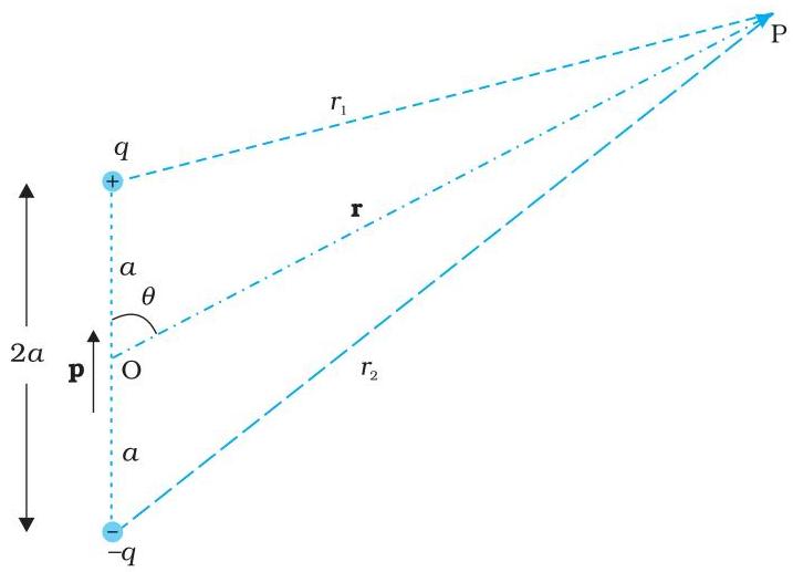FIGURE 2.5 Quantities involved in the calculation of potential due to a dipole.

Consistent with our prior methodology, the origin of our coordinate system is positioned at the dipole's center. It is established that the electric field adheres to the superposition principle. Given that potential is intrinsically linked to the work performed by the field, it logically follows that electrostatic potential similarly conforms to the superposition principle. Consequently, the total potential generated by the dipole is the algebraic sum of the potentials originating from the individual charges, $q$ and $-q$.

$ V = \frac {1}{4 \pi \varepsilon_ {0}} \left(\frac {q}{r _ {1}} - \frac {q}{r _ {2}}\right) \tag {2.9} $

where $r_1$ and $r_2$ denote the respective distances from the point $\mathbf{P}$ to the charges $q$ and $-q$.

Utilizing geometric principles,

$ r _ {1} ^ {2} = r ^ {2} + a ^ {2} - 2 a r \cos \theta $

$ r _ {2} ^ {2} = r ^ {2} + a ^ {2} + 2 a r \cos \theta \tag {2.10} $

Assuming that $r$ is significantly larger than $a$ (i.e., $r \gg a$), we shall retain only those terms up to the first order involving the ratio $a/r$.

$ \begin{array}{l} r _ {1} ^ {2} = r ^ {2} \left(1 - \frac {2 a \cos \theta}{r} + \frac {a ^ {2}}{r ^ {2}}\right) \ \equiv r ^ {2} \left(1 - \frac {2 a \cos \theta}{r}\right) \tag {2.11} \ \end{array} $

Similarly,

$ r _ {2} ^ {2} \equiv r ^ {2} \left(1 + \frac {2 a \cos \theta}{r}\right) \tag {2.12} $

By applying the Binomial theorem, and considering only terms up to the first order in the ratio $a/r$, we derive the following approximations:

$ \frac {1}{r _ {1}} \cong \frac {1}{r} \left(1 - \frac {2 a \cos \theta}{r}\right) ^ {- 1 / 2} \cong \frac {1}{r} \left(1 + \frac {a}{r} \cos \theta\right) \tag {2.13(a)} $

$ \frac {1}{r _ {2}} \cong \frac {1}{r} \left(1 + \frac {2 a \cos \theta}{r}\right) ^ {- 1 / 2} \cong \frac {1}{r} \left(1 - \frac {a}{r} \cos \theta\right) \tag {2.13(b)} $

Employing Equations (2.9) and (2.13), along with the definition $p = 2qa$, yields:

$ V = \frac {q}{4 \pi \varepsilon_ {0}} \frac {2 a \cos \theta}{r ^ {2}} = \frac {p \cos \theta}{4 \pi \varepsilon_ {0} r ^ {2}} \tag {2.14} $

Furthermore, the product $p\cos \theta$ can be represented vectorially as $\mathbf{p} \cdot \hat{\mathbf{r}}$

Here, $\hat{\mathbf{r}}$ denotes the unit vector oriented along the position vector $\mathbf{OP}$

Consequently, the electric potential attributable to a dipole is expressed as:

$ V = \frac{1}{4\pi\varepsilon_0} \frac{\mathbf{p} \cdot \hat{\mathbf{r}}}{r^2}; \quad (r \gg a) \tag{2.15} $

As noted, Equation (2.15) provides an approximate value, valid exclusively when the distance is considerably greater than the dipole's physical dimension, thereby allowing the neglect of higher-order terms involving $a/r$. Nevertheless, for a theoretical point dipole $\mathbf{p}$ situated at the origin, Equation (2.15) holds precisely.

Derived from Equation (2.15), the potential along the dipole's axis (where $\theta = 0$ or $\pi$) is expressed as:

$ V = \pm \frac{1}{4\pi\varepsilon_0} \frac{p}{r^2} \tag{2.16} $

(The positive value corresponds to $\theta = 0$, while the negative value applies for $\theta = \pi$.) In the equatorial plane, defined by $\theta = \pi/2$, the potential is identically zero.

Key distinctions between the electric potential generated by a dipole and that originating from a solitary point charge are evident upon comparing Equations (2.8) and (2.15):

(i) The potential generated by a dipole is contingent not merely on the radial distance $r$, but additionally on the angular separation between the position vector $\mathbf{r}$ and the dipole moment vector $\mathbf{p}$. (Despite this, it exhibits axial symmetry around $\mathbf{p}$. Specifically, if the position vector $\mathbf{r}$ is revolved around $\mathbf{p}$ while maintaining a constant $\theta$, all points $\mathbf{P}$ on the resultant conical surface will possess an identical potential to that at the initial point $\mathbf{P}$.)

(ii) At substantial distances, the electric potential of a dipole diminishes proportionally to $1/r^2$, in contrast to the $1/r$ dependence characteristic of the potential produced by a single charge. (For illustrative comparisons of $1/r^2$ versus $r$ and $1/r$ versus $r$ graphs, albeit presented in a different context, consult Figure 2.5.)

2.5 POTENTIAL DUE TO A SYSTEM OF CHARGES

Consider a system of charges $q_1, q_2, \ldots, q_n$ with position vectors $\mathbf{r}_1, \mathbf{r}_2, \ldots, \mathbf{r}_n$ relative to some origin (Fig. 2.6). The potential $V_1$ at $\mathbf{P}$ due to the charge $q_1$ is

$ V_1 = \frac{1}{4\pi\varepsilon_0} \frac{q_1}{r_{\mathrm{1P}}} $

where $r_{1\mathrm{P}}$ is the distance between $q_{1}$ and $\mathbf{P}$.

Similarly, the potential $V_2$ at $\mathbf{P}$ due to $q_2$ and $V_3$ due to $q_3$ are given by

$ V_2 = \frac{1}{4\pi\varepsilon_0} \frac{q_2}{r_{2\mathrm{P}}}, \quad V_3 = \frac{1}{4\pi\varepsilon_0} \frac{q_3}{r_{3\mathrm{P}}} $

where $r_{2\mathrm{P}}$ and $r_{3\mathrm{P}}$ are the distances of $\mathbf{P}$ from charges $q_2$ and $q_3$, respectively; and so on for the potential due to other charges. By the superposition principle, the potential $V$ at $\mathbf{P}$ due to the total charge configuration is the algebraic sum of the potentials due to the individual charges

$ V = V_1 + V_2 + \dots + V_n \tag{2.17} $

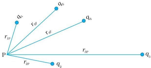FIGURE 2.6 Potential at a point due to a system of charges is the sum of potentials due to individual charges.

$ = \frac {1}{4 \pi \varepsilon_ {0}} \left(\frac {q _ {1}}{r _ {\mathrm {1 P}}} + \frac {q _ {2}}{r _ {2 \mathrm {P}}} + \dots \dots + \frac {q _ {n}}{r _ {n \mathrm {P}}}\right) \tag {2.18} $

If we have a continuous charge distribution characterised by a charge density $\rho (\mathbf{r})$, we divide it, as before, into small volume elements each of size $\Delta v$ and carrying a charge $\rho \Delta v$. We then determine the potential due to each volume element and sum (strictly speaking, integrate) over all such contributions, and thus determine the potential due to the entire distribution.

We have seen in Chapter 1 that for a uniformly charged spherical shell, the electric field outside the shell is as if the entire charge is concentrated at the centre. Thus, the potential outside the shell is given by

$ V = \frac {1}{4 \pi \varepsilon_ {0}} \frac {q}{r} \quad (r \geq R) \tag {2.19(a)} $

where $q$ is the total charge on the shell and $R$ its radius. The electric field inside the shell is zero. This implies (Section 2.6) that potential is constant inside the shell (as no work is done in moving a charge inside the shell), and, therefore, equals its value at the surface, which is

$ V = \frac {1}{4 \pi \varepsilon_ {0}} \frac {q}{R} \tag {2.19(b)} $

Example 2.2 Two charges $3 \times 10^{-8}$ C and $-2 \times 10^{-8}$ C are located $15\mathrm{cm}$ apart. At what point on the line joining the two charges is the electric potential zero? Take the potential at infinity to be zero.

Solution Let us take the origin O at the location of the positive charge. The line joining the two charges is taken to be the $x$-axis; the negative charge is taken to be on the right side of the origin (Fig. 2.7).

FIGURE 2.7

Let $\mathrm{P}$ be the required point on the $x$-axis where the potential is zero. If $x$ is the $x$-coordinate of $\mathrm{P}$, obviously $x$ must be positive. (There is no possibility of potentials due to the two charges adding up to zero for $x < 0$.) If $x$ lies between O and A, we have

$ \frac {1}{4 \pi \varepsilon_ {0}} \left[ \frac {3 \times 1 0 ^ {- 8}}{x \times 1 0 ^ {- 2}} - \frac {2 \times 1 0 ^ {- 8}}{(1 5 - x) \times 1 0 ^ {- 2}} \right] = 0 $

where $x$ is in cm. That is,

$ \frac {3}{x} - \frac {2}{1 5 - x} = 0 $

which gives $x = 9$ cm.

If $x$ lies on the extended line OA, the required condition is

$ \frac {3}{x} - \frac {2}{x - 1 5} = 0 $

which gives

$ x = 45 \text{ cm} $

Thus, electric potential is zero at $9 \text{ cm}$ and $45 \text{ cm}$ away from the positive charge on the side of the negative charge. Note that the formula for potential used in the calculation required choosing potential to be zero at infinity.

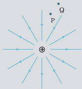
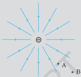
Example 2.3 Figures 2.8 (a) and (b) show the field lines of a positive and negative point charge respectively.

(a)

(b) FIGURE 2.8

(a) Give the signs of the potential difference $V_{\mathrm{P}} - V_{\mathrm{Q}}: V_{\mathrm{B}} - V_{\mathrm{A}}$ (b) Give the sign of the potential energy difference of a small negative charge between the points Q and P; A and B. (c) Give the sign of the work done by the field in moving a small positive charge from Q to P. (d) Give the sign of the work done by the external agency in moving a small negative charge from B to A. (e) Does the kinetic energy of a small negative charge increase or decrease in going from B to A?

Solution

(a) Given the inverse relationship between potential and radial distance ($V \propto \frac{1}{r}$), the potential at P ($V_{\mathrm{P}}$) exceeds that at Q ($V_{\mathrm{Q}}$), resulting in a positive value for $(V_{\mathrm{P}} - V_{\mathrm{Q}})$. Concurrently, $V_{B}$ is algebraically greater than $V_{A}$ (as $V_{B}$ is less negative), which implies that $(V_{B} - V_{A})$ is also positive. (b) A diminutive negative charge experiences attraction towards a positive charge. Consequently, such a charge transitions from a state of elevated potential energy to one of diminished potential energy. Therefore, for a small negative charge, the potential energy difference between Q and P is positive. Analogously, $(\mathrm{P.E.}){\mathrm{A}}$ is greater than $(\mathrm{P.E.}){\mathrm{B}}$, leading to a positive sign for the associated potential energy difference. (c) To transport a small positive charge from point Q to point P, an external agent must perform work in opposition to the electric field. Hence, the work performed by the electric field itself is negative. (d) When a small negative charge is displaced from B to A, the work expended by an external agency is positive. (e) The repulsive force acting upon the negative charge causes a reduction in its velocity, consequently diminishing its kinetic energy during its movement from B to A.

(a)

(b)

2.6 EQUIPOTENTIAL SURFACES

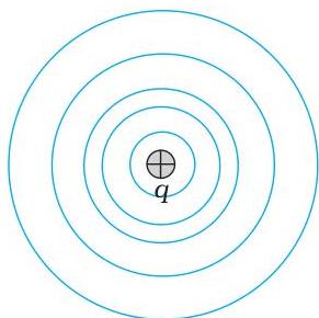
A surface upon which the electric potential maintains a constant value across all its points is defined as an equipotential surface. For an isolated charge $q$, the electric potential is determined by Eq. (2.8) as:

$ V = \frac {1}{4 \pi \varepsilon_ {o}} \frac {q}{r} $

This equation indicates that $V$ remains constant if $r$ is constant. Consequently, equipotential surfaces associated with a single point charge are concentric spherical shells centered at the charge's location.

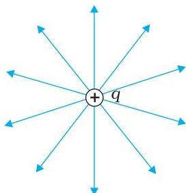
The electric field lines emanating from a single charge $q$ are radial, either originating from the charge or terminating at it, depending on whether $q$ is positive or negative, respectively. It is self-evident that the electric field at any given point is oriented perpendicularly to the equipotential surface passing through that point. This principle applies generally; for any configuration of charges, the equipotential surface at a specific point will always be normal to the electric field at that same point. The justification for this property is straightforward.

If the electric field were not perpendicular to the equipotential surface, it would possess a non-zero component tangential to the surface. Moving a unit test charge against the direction of this tangential field component would necessitate the performance of work. However, this contradicts the very definition of an equipotential surface, which dictates that there is no potential difference between any two points on the surface, and thus, no work is required to transport a test charge along it. Therefore, the electric field must, by necessity, be normal to the equipotential surface at every point. Beyond the portrayal offered by electric field lines, equipotential surfaces provide an alternative visual representation of charge configurations.

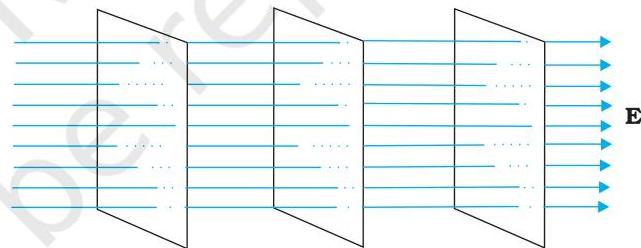
FIGURE 2.9 For a single charge $q$ (a) equipotential surfaces are spherical surfaces centred at the charge, and (b) electric field lines are radial, starting from the charge if $q > 0$. FIGURE 2.10 Equipotential surfaces for a uniform electric field.

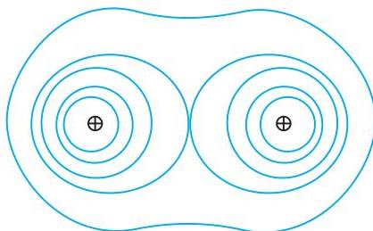
In the context of a uniform electric field $\mathbf{E}$, for example, one directed along the $x$-axis, the corresponding equipotential surfaces are planes orthogonal to the $x$-axis, meaning they are planes parallel to the $y-z$ plane (as depicted in Fig. 2.10). Equipotential surfaces for (a) an electric dipole and (b) two identical positive charges are illustrated in Fig. 2.11.

(a)

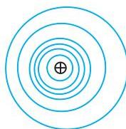FIGURE 2.11 Some equipotential surfaces for (a) a dipole, (b) two identical positive charges.

(b)

2.6.1 Relation between field and potential

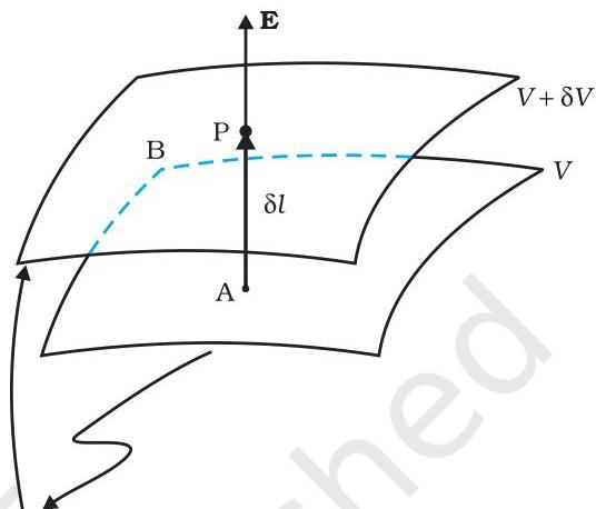
Let's examine the relationship using two infinitesimally separated equipotential surfaces, designated A and B (Fig. 2.12), possessing electric potential values of $V$ and $V + \delta V$, respectively. Here, $\delta V$ represents the alteration in potential $V$ along the direction of the electric field $\mathbf{E}$. Consider point P situated on surface B. The distance $\delta l$ denotes the perpendicular separation from surface A to point P. If a unit positive test charge were to be displaced along this perpendicular path from surface B to surface A, opposing the electric field's direction, the work expended during this displacement would be $|\mathbf{E}| \delta l$.

This work corresponds precisely to the potential difference $V_{A} - V_{B'}$.

Thus,

$ | \mathbf {E} | \delta l = V - (V + \delta V) = - \delta V $

$ \text{i.e., } | \mathbf {E} | = - \frac {\delta V}{\delta l} \tag {2.20} $

Given that $\delta V$ signifies a decrease in potential, making it inherently negative (i.e., $\delta V = -|\delta V|$), Equation (2.20) can be reformulated as:

Equipotentials FIGURE 2.12 From the potential to the field.

$ \left| \mathbf {E} \right| = - \frac {\delta V}{\delta l} = + \frac {\left| \delta V \right|}{\delta l} \tag {2.21} $

Consequently, two fundamental principles emerge regarding the interrelationship between the electric field and electric potential:

(i) The electric field vector points in the direction of the most rapid decrease in electric potential. (ii) Its magnitude is defined by the rate of change of the potential's magnitude per unit displacement, measured perpendicularly to the equipotential surface at that specific location.

2.7 POTENTIAL ENERGY OF A SYSTEM OF CHARGES

Consider first the simple case of two charges $q_{1}$ and $q_{2}$ with position vector $\mathbf{r}{1}$ and $\mathbf{r}{2}$ relative to some origin. Let us calculate the work done (externally) in building up this configuration. This means that we consider the charges $q_{1}$ and $q_{2}$ initially at infinity and determine the work done by an external agency to bring the charges to the given locations. Suppose, first the charge $q_{1}$ is brought from infinity to the point $\mathbf{r}{1}$. There is no external field against which work needs to be done, so work done in bringing $q{1}$ from infinity to $\mathbf{r}_{1}$ is zero. This charge produces a potential in space given by

$ V _ {1} = \frac {1}{4 \pi \varepsilon_ {0}} \frac {q _ {1}}{r _ {1 P}} $

where $r_{1P}$ is the distance of a point $P$ in space from the location of $q_{1}$. From the definition of potential, work done in bringing charge $q_{2}$ from infinity to the point $\mathbf{r}{2}$ is $q{2}$ times the potential at $\mathbf{r}{2}$ due to $q{1}$:

Work done on $q_{2}$ = $ \frac{1}{4\pi\varepsilon_{0}}\frac{q_{1}q_{2}}{r_{12}}

$

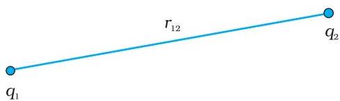FIGURE 2.13 Potential energy of a system of charges $q_{1}$ and $q_{2}$ is directly proportional to the product of charges and inversely to the distance between them.

where $r_{12}$ is the distance between points 1 and 2.

Since electrostatic force is conservative, this work gets stored in the form of potential energy of the system. Thus, the potential energy of a system of two charges $q_{1}$ and $q_{2}$ is

$ U = \frac {1}{4 \pi \varepsilon_ {0}} \frac {q _ {1} q _ {2}}{r _ {1 2}} \tag {2.22} $

Obviously, if $q_{2}$ was brought first to its present location and $q_{1}$ brought later, the potential energy $U$ would be the same.

More generally, the potential energy expression,

Eq. (2.22), is unaltered whatever way the charges are brought to the specified locations, because of path-independence of work for electrostatic force.

Equation (2.22) is true for any sign of $q_{1}$ and $q_{2}$. If $q_{1}q_{2} > 0$, potential energy is positive. This is as expected, since for like charges $(q_{1}q_{2} > 0)$, electrostatic force is repulsive and a positive amount of work is needed to be done against this force to bring the charges from infinity to a finite distance apart. For unlike charges $(q_{1}q_{2} < 0)$, the electrostatic force is attractive. In that case, a positive amount of work is needed against this force to take the charges from the given location to infinity. In other words, a negative amount of work is needed for the reverse path (from infinity to the present locations), so the potential energy is negative.

Equation (2.22) is easily generalised for a system of any number of point charges. Let us calculate the potential energy of a system of three charges $q_{1}$, $q_{2}$ and $q_{3}$ located at $\mathbf{r}_1, \mathbf{r}_2, \mathbf{r}3$, respectively. To bring $q{1}$ first from infinity to $\mathbf{r}1$, no work is required. Next we bring $q{2}$ from infinity to $\mathbf{r}_2$. As before, work done in this step is

$ q _ {2} V _ {1} \left(\mathbf {r} _ {2}\right) = \frac {1}{4 \pi \varepsilon_ {0}} \frac {q _ {1} q _ {2}}{r _ {1 2}} \tag {2.23} $

The electrostatic potential generated by charges $q_1$ and $q_2$ at an arbitrary location $P$ is expressed as:

$ V _ {1, 2} = \frac {1}{4 \pi \varepsilon_ {0}} \left(\frac {q _ {1}}{r _ {1 P}} + \frac {q _ {2}}{r _ {2 P}}\right) \tag {2.24} $

Subsequently, the work expended to transport charge $q_3$ from an infinite distance to position $\mathbf{r}3$ is calculated as the product of $q_3$ and the potential $V{1,2}$ evaluated at $\mathbf{r}_3$.

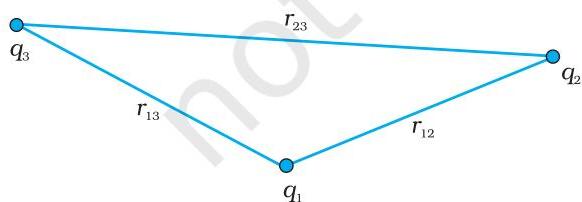FIGURE 2.14 Potential energy of a system of three charges is given by Eq. (2.26), with the notation given in the figure.

$ q _ {3} V _ {1, 2} \left(\mathbf {r} _ {3}\right) = \frac {1}{4 \pi \varepsilon_ {0}} \left(\frac {q _ {1} q _ {3}}{r _ {1 3}} + \frac {q _ {2} q _ {3}}{r _ {2 3}}\right) \tag {2.25} $

The cumulative work required to establish this arrangement of charges at their specified positions is determined by summing the individual work contributions from each step, as detailed in Eq. (2.23) and Eq. (2.25):

$ U = \frac {1}{4 \pi \varepsilon_ {0}} \left(\frac {q _ {1} q _ {2}}{r _ {1 2}} + \frac {q _ {1} q _ {3}}{r _ {1 3}} + \frac {q _ {2} q _ {3}}{r _ {2 3}}\right) \tag {2.26} $

Due to the inherent conservative property of the electrostatic force (or, synonymously, the path-independent nature of the work performed), the ultimate formulation for $U$, as presented in Eq. (2.26), does not depend on the specific sequence used to construct the charge configuration. This potential energy solely reflects the current state of the configuration, rather than the process by which that state was attained.

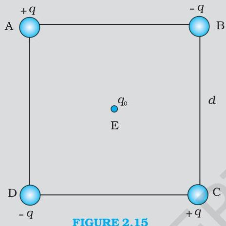
Example 2.4 Four discrete charges are positioned at the vertices of a square, labeled ABCD, with side length $d$, as depicted in Fig. 2.15(a). (a) Determine the work necessary to establish this particular arrangement. (b) Subsequently, an additional charge $q_0$ is introduced to the geometric center E of the square, while the initial four charges remain fixed at their corner locations. Calculate the supplementary work required for this action.

Solution

(a) The work expended in assembling a system of charges is solely contingent upon their final spatial configuration, irrespective of the specific path or sequence of assembly. Consequently, to determine this work, we can elect a particular sequence for positioning the charges at locations A, B, C, and D. Let us assume the charge $+q$ is first positioned at A, followed by the sequential placement of charges $-q$, $+q$, and $-q$ at B, C, and D, respectively. The aggregate work required can be computed through a series of incremental steps:

(i) The work required to introduce the charge $+q$ to position A, given an initially charge-free environment, is zero.

(ii) The work associated with placing the charge $-q$ at location B, subsequent to the placement of $+q$ at A, is determined by the product of the charge at B and the electrostatic potential existing at B due to the charge $+q$ at A: $ = - q \times \left(\frac {q}{4 \pi \varepsilon_ {0} d}\right) = - \frac {q ^ {2}}{4 \pi \varepsilon_ {0} d} $

(iii) The work required to position the charge $+q$ at C, with charges $+q$ already at A and $-q$ at B, is computed as the charge at C multiplied by the electrostatic potential at C resulting from the charges at A and B: $ \begin{array}{l} = + q \left(\frac {+ q}{4 \pi \varepsilon_ {0} d \sqrt {2}} + \frac {- q}{4 \pi \varepsilon_ {0} d}\right) \ = \frac {- q ^ {2}}{4 \pi \varepsilon_ {0} d} \left(1 - \frac {1}{\sqrt {2}}\right) \ \end{array} $

(iv) The work necessary to introduce the charge $-q$ to D, given the presence of $+q$ at A, $-q$ at B, and $+q$ at C, is determined by the charge at D multiplied by the potential at D generated by the charges at A, B, and C: $ \begin{array}{l} = - q \left(\frac {+ q}{4 \pi \varepsilon_ {0} d} + \frac {- q}{4 \pi \varepsilon_ {0} d \sqrt {2}} + \frac {q}{4 \pi \varepsilon_ {0} d}\right) \ = \frac {- q ^ {2}}{4 \pi \varepsilon_ {0} d} \left(2 - \frac {1}{\sqrt {2}}\right) \ \end{array} $

Summing the work contributions from steps (i), (ii), (iii), and (iv) yields the total work necessary for this configuration: $ \begin{array}{l} = \frac {- q ^ {2}}{4 \pi \varepsilon_ {0} d} \left{(0) + (1) + \left(1 - \frac {1}{\sqrt {2}}\right) + \left(2 - \frac {1}{\sqrt {2}}\right) \right} \ = \frac {- q ^ {2}}{4 \pi \varepsilon_ {0} d} (4 - \sqrt {2}) \end{array} $ This work, fundamentally dependent solely on the ultimate spatial arrangement of the charges rather than their assembly process, constitutes the system's total electrostatic potential energy by definition.

(Learners are encouraged to compute this work/energy using an alternative sequence of charge placement to empirically verify the invariance of the total energy.)

(b) The additional work required to transport a charge $q_{0}$ to point E, given the existing configuration of four charges at A, B, C, and D, is expressed as $q_{0} \times$ (the electrostatic potential at E resulting from the charges at A, B, C, and D). It is evident that the net electrostatic potential at E is zero, as the potentials contributed by charges at A and C are precisely counteracted by those from charges at B and D. Consequently, no external work is needed to introduce any charge to point E.

2.8 POTENTIAL ENERGY IN AN EXTERNAL FIELD

2.8.1 Potential energy of a single charge

In Section 2.7, the source of the electric field was specified – the charges and their locations – and the potential energy of the system of those charges was determined. In this section, we ask a related but a distinct question. What is the potential energy of a charge $q$ in a given field? This question was, in fact, the starting point that led us to the notion of the electrostatic potential (Sections 2.1 and 2.2). But here we address this question again to clarify in what way it is different from the discussion in Section 2.7.

The main difference is that we are now concerned with the potential energy of a charge (or charges) in an external field. The external field $\mathbf{E}$ is not produced by the given charge(s) whose potential energy we wish to calculate. $\mathbf{E}$ is produced by sources external to the given charge(s). The external sources may be known, but often they are unknown or unspecified; what is specified is the electric field $\mathbf{E}$ or the electrostatic potential $V$ due to the external sources. We assume that the charge $q$ does not significantly affect the sources producing the external field. This is true if $q$ is very small, or the external sources are held fixed by other unspecified forces. Even if $q$ is finite, its influence on the external sources may still be ignored in the situation when very strong sources far away at infinity produce a finite field $\mathbf{E}$ in the region of interest. Note again that we are interested in determining the potential energy of a given charge $q$ (and later, a system of charges) in the external field; we are not interested in the potential energy of the sources producing the external electric field.

The external electric field $\mathbf{E}$ and the corresponding external potential $V$ may vary from point to point. By definition, $V$ at a point $P$ is the work done in bringing a unit positive charge from infinity to the point $P$.

(We continue to take potential at infinity to be zero.) Thus, work done in bringing a charge $q$ from infinity to the point $P$ in the external field is $qV$. This work is stored in the form of potential energy of $q$. If the point $P$ has position vector $\mathbf{r}$ relative to some origin, we can write:

Potential energy of $q$ at $\mathbf{r}$ in an external field

$ = q V (\mathbf {r}) \tag {2.27} $

where $V(\mathbf{r})$ is the external potential at the point $\mathbf{r}$.

Thus, if an electron with charge $q = e = 1.6 \times 10^{-19}$ C is accelerated by a potential difference of $\Delta V = 1$ volt, it would gain energy of $q\Delta V = 1.6 \times 10^{-19}$ J. This unit of energy is defined as 1 electron volt or 1eV, i.e., $1 \mathrm{eV} = 1.6 \times 10^{-19}$ J. The units based on eV are most commonly used in atomic, nuclear and particle physics, (1 keV = 10³eV = 1.6 × 10⁻¹⁶J, 1 MeV = 10⁶eV = 1.6 × 10⁻¹³J, 1 GeV = 10⁹eV = 1.6 × 10⁻¹⁰J and 1 TeV = 10¹²eV = 1.6 × 10⁻⁷J). [This has already been defined on Page 117, XI Physics Part I, Table 6.1.]

2.8.2 Potential energy of a system of two charges in an external field

To determine the potential energy associated with a system comprising two charges, $q_{1}$ and $q_{2}$, situated at positions $\mathbf{r}{1}$ and $\mathbf{r}{2}$ respectively, within an external field, we consider the total work expended in assembling this configuration. Initially, the work required to transport charge $q_{1}$ from an infinite distance to its designated position $\mathbf{r}{1}$ is $q{1}V(\mathbf{r}{1})$, as established by Eq. (2.27). Subsequently, when bringing charge $q{2}$ to its location $\mathbf{r}{2}$, the work performed must overcome not only the influence of the external electric field $\mathbf{E}$ but also the electric field generated by $q{1}$.

Work done on $q_{2}$ against the external field $ = q _ {2} V \left(\mathbf {r} _ {2}\right) $

Work done on $q_{2}$ against the field due to $q_{1}$ $ = \frac {q _ {1} q _ {2}}{4 \pi \varepsilon_ {0} r _ {1 2}} $

Here, $r_{12}$ denotes the separation distance between $q_1$ and $q_2$. Drawing upon Eqs. (2.27) and (2.22), and applying the principle of superposition for electric fields, the cumulative work required to position $q_2$ against both the external field and the field from $q_1$ is computed as:

Work done in bringing $q_{2}$ to $\mathbf{r}2$ $ = q _ {2} V \left(\mathbf {r} _ {2}\right) + \frac {q _ {1} q _ {2}}{4 \pi \varepsilon {0} r _ {1 2}} \tag {2.28} $

Consequently, the potential energy of the entire system is equivalent to the total work invested in establishing this charge arrangement:

Potential energy of the system = the total work done in assembling the configuration $ = q _ {1} V \left(\mathbf {r} _ {1}\right) + q _ {2} V \left(\mathbf {r} _ {2}\right) + \frac {q _ {1} q _ {2}}{4 \pi \varepsilon_ {0} r _ {1 2}} \tag {2.29} $

Example 2.5

(a) Determine the electrostatic potential energy of a system consisting of two charges $7\mu \mathrm{C}$ and $-2\mu \mathrm{C}$ (and with no external field) placed at $(-9\mathrm{cm},0,0)$ and $(9\mathrm{cm},0,0)$ respectively. (b) How much work is required to separate the two charges infinitely away from each other?

(c) Suppose that the same system of charges is now placed in an external electric field $E = A(1 / r^2)$; $A = 9 \times 10^{5} , \mathrm{NC}^{-1} , \mathrm{m}^{2}$. What would the electrostatic energy of the configuration be?

Solution

(a) $U = \frac{1}{4\pi\varepsilon_0}\frac{q_1q_2}{r} = 9\times 10^9\times \frac{7\times(-2)\times 10^{-12}}{0.18} = -0.7\mathrm{J}.$ (b) $W = U_{2} - U_{1} = 0 - U = 0 - (-0.7) = 0.7\mathrm{J}.$ (c) The mutual interaction energy of the two charges remains unchanged. In addition, there is the energy of interaction of the two charges with the external electric field. We find,

$ q _ {1} V \left(\mathbf {r} _ {1}\right) + q _ {2} V \left(\mathbf {r} _ {2}\right) = A \frac {7 \mu \mathrm {C}}{0 . 0 9 \mathrm {m}} + A \frac {- 2 \mu \mathrm {C}}{0 . 0 9 \mathrm {m}} $

and the net electrostatic energy is

$ \begin{array}{l} q _ {1} V \left(\mathbf {r} _ {1}\right) + q _ {2} V \left(\mathbf {r} _ {2}\right) + \frac {q _ {1} q _ {2}}{4 \pi \varepsilon_ {0} r _ {1 2}} = A \frac {7 \mu \mathrm {C}}{0 . 0 9 \mathrm {m}} + A \frac {- 2 \mu \mathrm {C}}{0 . 0 9 \mathrm {m}} - 0. 7 \mathrm {J} \ = 7 0 - 2 0 - 0. 7 = 4 9. 3 \mathrm {J} \ \end{array} $

2.8.3 Potential energy of a dipole in an external field

Consider a dipole with charges $q_{1} = +q$ and $q_{2} = -q$ placed in a uniform electric field $\mathbf{E}$, as shown in Fig. 2.16.

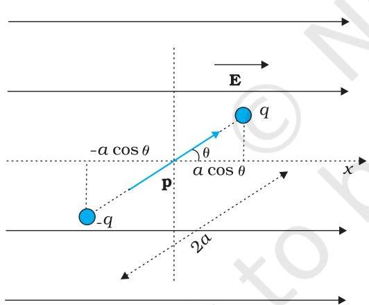FIGURE 2.16 Potential energy of a dipole in a uniform external field.

As seen in the last chapter, in a uniform electric field, the dipole experiences no net force; but experiences a torque $\tau$ given by

$ \tau = \mathbf {p} \times \mathbf {E} \tag {2.30} $

which will tend to rotate it (unless $\mathbf{p}$ is parallel or antiparallel to $\mathbf{E}$). Suppose an external torque $\tau_{\mathrm{ext}}$ is applied in such a manner that it just neutralises this torque and rotates it in the plane of paper from angle $\theta_0$ to angle $\theta_{1}$ at an infinitesimal angular speed and without angular acceleration. The amount of work done by the external torque will be given by

$ \begin{array}{l} W = \int_ {\theta_ {0}} ^ {\theta_ {1}} t _ {\text {e x t}} (\theta) d \theta = \int_ {\theta_ {0}} ^ {\theta_ {1}} p E \sin \theta d \theta \ = p E \left(\cos \theta_ {0} - \cos \theta_ {1}\right) \tag {2.31} \ \end{array} $

This work is stored as the potential energy of the system. We can then associate potential energy $U(\theta)$ with an inclination $\theta$ of the dipole. Similar to other potential energies, there is a freedom in choosing the angle where the potential energy $U$ is taken to be zero. A natural choice is to take $\theta_0 = \pi / 2$. (An explanation for it is provided towards the end of discussion.) We can then write,

$ U (\theta) = p E \left(\cos \frac {\pi}{2} - \cos \theta\right) = p E \cos \theta = - \mathbf {p}. \mathbf {E} \tag {2.32} $

This expression can alternately be understood also from Eq. (2.29). We apply Eq. (2.29) to the present system of two charges $+q$ and $-q$. The potential energy expression then reads

$ U'(\theta) = q \left[ V(\mathbf{r}_1) - V(\mathbf{r}_2) \right] - \frac{q^2}{4\pi\varepsilon_0 \times 2\alpha} \tag{2.33} $

Here, $\mathbf{r}_1$ and $\mathbf{r}_2$ denote the position vectors of $+q$ and $-q$. Now, the potential difference between positions $\mathbf{r}_1$ and $\mathbf{r}_2$ equals the work done in bringing a unit positive charge against field from $\mathbf{r}_2$ to $\mathbf{r}_1$. The displacement parallel to the force is $2\alpha \cos \theta$. Thus, $[V(\mathbf{r}_1) - V(\mathbf{r}_2)] = -E \times 2\alpha \cos \theta$. We thus obtain,

$ U'(\theta) = -pE \cos \theta - \frac{q^2}{4\pi\varepsilon_0 \times 2\alpha} = -\mathbf{p} \cdot \mathbf{E} - \frac{q^2}{4\pi\varepsilon_0 \times 2\alpha} \tag{2.34} $

We note that $U'(\theta)$ differs from $U(\theta)$ by a quantity which is just a constant for a given dipole. Since a constant is insignificant for potential energy, we can drop the second term in Eq. (2.34) and it then reduces to Eq. (2.32).

The rationale for setting $\theta_0 = \pi/2$ becomes clear. In this specific configuration, the work required to move charge $+q$ and charge $-q$ against the external field $\mathbf{E}$ perfectly counteracts itself, as these work components are equal in magnitude and opposite in sign. Consequently, the net work, expressed as $q[V(\mathbf{r}_1) - V(\mathbf{r}_2)]$, is zero.

Example 2.6 Consider a substance where each molecule possesses a permanent electric dipole moment with a magnitude of $10^{-29}$ C m. A single mole of this material undergoes polarization (under low-temperature conditions) when subjected to a powerful electrostatic field of $10^6$ V m$^{-1}$. If the field's orientation abruptly shifts by $60^\circ$, determine the quantity of heat dissipated by the substance as its dipoles reorient to align with the new field direction. For calculation simplicity, assume the sample is $100%$ polarized.

Solution The dipole moment associated with each individual molecule is given as $10^{-29}$ C m.

Considering that one mole of the substance comprises $6 \times 10^{23}$ molecules,

The aggregate dipole moment for all molecules, $p$, is computed as: $p = 6 \times 10^{23} \times 10^{-29}$ C m

$ = 6 \times 10^{-6} \text{C m} $

The initial potential energy, $U_l$, is determined using the formula: $U_l = -pE \cos \theta = -6 \times 10^{-6} \times 10^6 \cos 0^\circ = -6$ J

The final potential energy (with $\theta$ set to $60^\circ$), $U_l$, is calculated as: $U_l = -6 \times 10^{-6} \times 10^6 \cos 60^\circ = -3$ J

The resulting alteration in potential energy is: -3 J - (-6J) = 3 J

Consequently, a reduction in potential energy occurs. This energy must therefore correspond to the heat liberated by the substance as its dipoles reorient into alignment.

2.9 ELECTROSTATICS OF CONDUCTORS

The concept of conductors and insulators was briefly introduced in Chapter 1. Conductors are distinguished by their possession of mobile charge carriers. In the case of metallic conductors, these carriers are electrons. Within a metal, the outer (valence) electrons dissociate from their parent atoms, becoming freely movable throughout the material. These electrons are confined within the metal's boundaries but are not free to exit it. These delocalized electrons behave somewhat like a gas, constantly colliding with each other and the fixed ion cores, resulting in random motion. Upon the application of an external electric field, they exhibit a net drift opposing the field's direction. Conversely, the positive ions, comprising the nuclei and bound electrons, remain fixed in their lattice positions. In contrast, electrolytic conductors utilize both positive and negative ions as charge carriers; however,

the dynamics in such instances are considerably more intricate, as the movement of these charge carriers is influenced both by the external electric field and by inherent chemical forces (as discussed in Chapter 3). For the scope of this discussion, we will confine our analysis to metallic solid conductors. Let us now examine significant principles pertaining to the electrostatics of conductors.

1. Inside a conductor, electrostatic field is zero

Consider a conductor, irrespective of whether it is neutral or charged. An external electrostatic field might also be present. In an electrostatic state, characterized by the absence of current flow either within or on the surface of the conductor, the electric field is uniformly zero throughout its interior. This characteristic can be regarded as the defining attribute of a conductor. Conductors possess mobile electrons. Should an electric field be non-zero, these free charge carriers would experience a force and consequently drift. In the static condition, these free charges redistribute themselves in such a manner that the electric field vanishes everywhere within the conductor. The electrostatic field is therefore zero inside a conductor.

2. At the surface of a charged conductor, electrostatic field must be normal to the surface at every point

If the electric field, $\mathbf{E}$, were not perpendicular to the surface, it would possess a non-zero component oriented along the surface. This tangential component would then exert a force on the free charges located on the conductor's surface, causing them to move. Consequently, in a static situation, $\mathbf{E}$ must not have any tangential component. Thus, the electrostatic field at the surface of a charged conductor is necessarily normal to the surface at every point. (Should a conductor lack any surface charge density, the field is zero even at its surface.) Refer to result 5.

3. The interior of a conductor can have no excess charge in the static situation

A conductor in its neutral state contains an equivalent quantity of positive and negative charges distributed uniformly throughout any infinitesimally small volume or surface region. Upon charging a conductor, any surplus charge is restricted to its exterior surface under static conditions. This principle is a direct consequence of Gauss's Law. To demonstrate this, let us consider an arbitrary infinitesimal volume element $v$ situated within the conductor's interior. Given that the electrostatic field is zero everywhere inside a conductor in equilibrium, it must also be zero across the closed surface $S$ that encloses $v$. Consequently, the total electric flux passing through $S$ must be zero. Applying Gauss's Law, it follows directly that no net charge is contained within $S$. Since the dimensions of the surface $S$ (and thus the volume $v$) can be arbitrarily reduced, approaching an infinitesimal size, this implies that no net charge exists at any point within the conductor's bulk, compelling any excess charge to reside solely on its outer boundary.

4. Electrostatic potential is constant throughout the volume of the conductor and has the same value (as inside) on its surface

This conclusion is derived from previously established principles (results 1 and 2). Given that the electric field $\mathbf{E} = 0$ throughout the interior of a conductor and possesses no tangential component along its surface, no work is expended when transporting a small test charge anywhere within the conductor's bulk or across its exterior. Consequently, no potential difference exists between any two arbitrary points located within or on the conductor's boundary. This directly substantiates the stated outcome. However, in the case of a charged conductor, an electric field normal to the surface is present; this implies that the potential at the surface itself will differ from the potential at a point immediately external to it.

When considering a system comprising multiple conductors, irrespective of their size, geometry, or charge distribution, each individual conductor will exhibit a constant potential value throughout its extent, though this constant may vary between different conductors in the system.

5. Electric field at the surface of a charged conductor

$ \mathbf {E} = \frac {\sigma}{\varepsilon_ {0}} \hat {\mathbf {n}} \tag {2.35} $

where $\sigma$ is the surface charge density and $\hat{\mathbf{n}}$ is a unit vector normal to the surface in the outward direction.

To derive the result, choose a pill box (a short cylinder) as the Gaussian surface about any point $P$ on the surface, as shown in Fig. 2.17. The pill box is partly inside and partly outside the surface of the conductor. It has a small area of cross section $\delta S$ and negligible height.

Just inside the surface, the electrostatic field is zero; just outside, the field is normal to the surface with magnitude $E$. Thus, the contribution to the total flux through the pill box comes only from the outside (circular) cross-section of the pill box. This equals $\pm E\delta S$ (positive for $\sigma > 0$, negative for $\sigma < 0$), since over the small area $\delta S$, $\mathbf{E}$ may be considered constant and $\mathbf{E}$ and $\delta S$ are parallel or antiparallel. The charge enclosed by the pill box is $\sigma\delta S$.

By Gauss's law

$ E \delta S = \frac {| \sigma | \delta S}{\varepsilon_ {0}} $

$ E = \frac {| \sigma |}{\varepsilon_ {0}} \tag {2.36} $

Including the fact that electric field is normal to the surface, we get the vector relation, Eq. (2.35), which is true for both signs of $\sigma$. For $\sigma > 0$, electric field is normal to the surface outward; for $\sigma < 0$, electric field is normal to the surface inward.

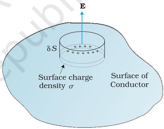FIGURE 2.17 The Gaussian surface (a pill box) chosen to derive Eq. (2.35) for electric field at the surface of a charged conductor.

6. Electrostatic shielding

Consider a conductor with a cavity, with no charges inside the cavity. A remarkable result is that the electric field inside the cavity is zero, whatever be the size and shape of the cavity and whatever be the charge on the conductor and the external fields in which it might be placed. We have proved a simple case of this result already: the electric field inside a charged spherical shell is zero. The proof of the result for the shell makes use of the spherical symmetry of the shell (see Chapter 1). But the vanishing of electric field in the (charge-free) cavity of a conductor is, as mentioned above, a very general result. A related result is that even if the conductor

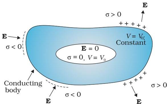FIGURE 2.18 The electric field inside a cavity of any conductor is zero. All charges reside only on the outer surface of a conductor with cavity. (There are no charges placed in the cavity.)

is charged or charges are induced on a neutral conductor by an external field, all charges reside only on the outer surface of a conductor with cavity.

The proofs of the results noted in Fig. 2.18 are omitted here, but we note their important implication. Whatever be the charge and field configuration outside, any cavity in a conductor remains shielded from outside electric influence: the field inside the cavity is always zero. This is known as electrostatic shielding. The effect can be made use of in protecting sensitive instruments from outside electrical influence. Figure 2.19 gives a summary of the important electrostatic properties of a conductor.

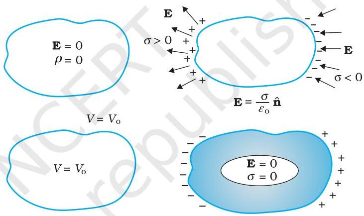FIGURE 2.19 Some important electrostatic properties of a conductor.

Example 2.7

(a) A comb run through one's dry hair attracts small bits of paper. Why? What happens if the hair is wet or if it is a rainy day? (Remember, a paper does not conduct electricity.) (b) Ordinary rubber is an insulator. But special rubber tyres of aircraft are made slightly conducting. Why is this necessary? (c) Vehicles carrying inflammable materials usually have metallic ropes touching the ground during motion. Why? (d) A bird perches on a bare high power line, and nothing happens to the bird. A man standing on the ground touches the same line and gets a fatal shock. Why?

Solution

(a) The phenomenon occurs because the comb acquires an electrical charge through the process of friction. This charged comb then induces polarization in the paper's molecules, leading to a net attractive force. However, in conditions of dampness, such as wet hair or high humidity, the frictional forces between the hair and the comb are significantly diminished. Consequently, the comb fails to accumulate a charge, thereby losing its ability to attract small paper fragments.

(b) This design facilitates the dissipation of electrical charge, which accumulates due to friction, directly into the ground. An excessive buildup of static electricity poses a risk of generating a spark, which could potentially ignite flammable materials. (c) Reason similar to (b). (d) Electrical current will only flow if there exists a potential difference between two points.

2.10 DIELECTRICS AND POLARISATION

Dielectrics are non-conducting substances. In contrast to conductors, they have no (or negligible number of) charge carriers. Recall from Section

2.9 what happens when a conductor is placed in an external electric field. The free charge carriers move and charge distribution in the conductor adjusts itself in such a way that the electric field due to induced charges opposes the external field within the conductor. This happens until, in the static situation, the two fields cancel each other and the net electrostatic field in the conductor is zero. In a dielectric, this free movement of charges is not possible. It turns out that the external field induces dipole moment by stretching or re-orienting molecules of the dielectric. The collective effect of all the molecular dipole moments is net charges on the surface of the dielectric which produce a field that opposes the external field. Unlike in a conductor, however, the opposing field so induced does not exactly cancel the external field. It only reduces it. The extent of the effect depends on the nature of the dielectric. To understand the effect, we need to look at the charge distribution of a dielectric at the molecular level.

The molecules of a substance may be polar or non-polar. In a non-polar molecule, the centres of positive and negative charges coincide. The molecule then has no permanent (or intrinsic) dipole moment. Examples of non-polar molecules are oxygen $(\mathrm{O}_2)$ and hydrogen $(\mathrm{H}_2)$ molecules which, because of their symmetry, have no dipole moment. On the other hand, a polar molecule is one in which the centres of positive and negative charges are separated (even when there is no external field). Such molecules have a permanent dipole moment. An ionic molecule such as HCl or a molecule of water $(\mathrm{H}_2\mathrm{O})$ are examples of polar molecules.

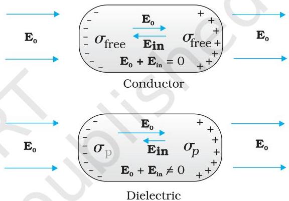FIGURE 2.20 Difference in behaviour of a conductor and a dielectric in an external electric field.

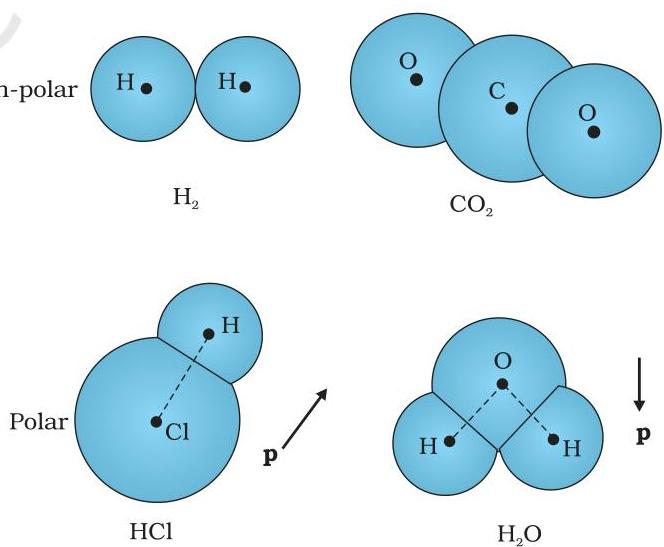FIGURE 2.21 Some examples of polar and non-polar molecules.

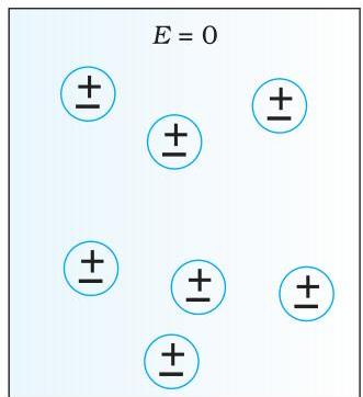(a) Non-polar molecules

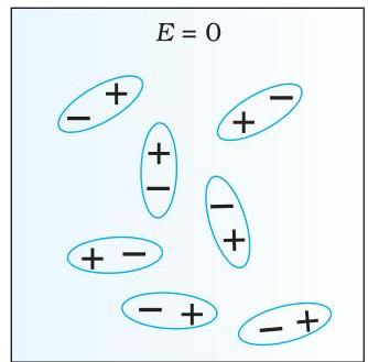(b) Polar molecules

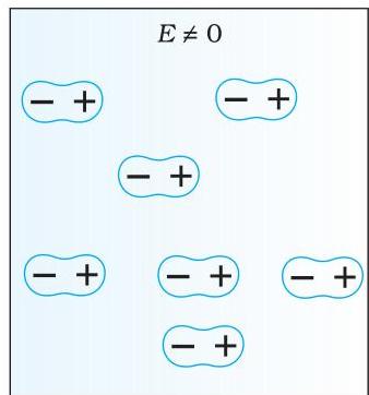
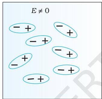FIGURE 2.22 A dielectric develops a net dipole moment in an external electric field. (a) Non-polar molecules, (b) Polar molecules.

In an external electric field, the positive and negative charges of a nonpolar molecule are displaced in opposite directions. The displacement stops when the external force on the constituent charges of the molecule is balanced by the restoring force (due to internal fields in the molecule). The non-polar molecule thus develops an induced dipole moment. The dielectric is said to be polarised by the external field. We consider only the simple situation when the induced dipole moment is in the direction of the field and is proportional to the field strength. (Substances for which this assumption is true are called linear isotropic dielectrics.) The induced dipole moments of different molecules add up giving a net dipole moment of the dielectric in the presence of the external field.

A dielectric material containing polar molecules also develops a net dipole moment when subjected to an external field, though the underlying mechanism differs. In the absence of an external field, the inherent permanent dipoles are randomly oriented due to thermal agitation, resulting in a zero net dipole moment. When an external field is applied, these individual dipole moments tend to align themselves with the field. Summed over all the molecules, this alignment produces a net dipole moment in the direction of the external field, thereby polarizing the dielectric. The degree of polarization is governed by the relative strengths of two opposing influences: the dipole potential energy in the external field, which promotes alignment, and the thermal energy, which tends to disrupt this alignment. An 'induced dipole moment' effect, similar to that observed in non-polar molecules, may also contribute, but the alignment of permanent dipoles is generally the more significant factor for polar molecules.

Thus, in both cases, whether the dielectric is composed of polar or non-polar molecules, a net dipole moment forms in the presence of an external field. The dipole moment per unit volume is termed polarization and is denoted by $\mathbf{P}$. For linear isotropic dielectrics,

$ \mathbf {P} = \varepsilon_ {0} \chi_ {e} \mathbf {E} \tag {2.37} $

where $\chi_{e}$ is a constant characteristic of the dielectric and is known as the electric susceptibility of the dielectric medium.

It is possible to establish a relationship between $\chi_{e}$ and the molecular properties of the substance, but we shall not pursue that here.

The question then arises: how does the polarized dielectric modify the original external field within its interior? For simplicity, let us consider a rectangular dielectric slab positioned in a uniform external field $\mathbf{E}_0$ parallel to two of its faces. This field induces a uniform polarization $\mathbf{P}$ throughout the dielectric. Consequently,

every volume element $\Delta v$ of the slab possesses a dipole moment $\mathbf{P} \Delta v$ aligned with the field. While macroscopically small, each volume element $\Delta v$ contains a very large number of molecular dipoles. Anywhere inside the dielectric, a volume element $\Delta v$ exhibits no net charge (though it does possess a net dipole moment). This is because the positive charge of one dipole is situated close to the negative charge of an adjacent dipole. However, at the surfaces of the dielectric oriented normal to the electric field, a net charge density is clearly present. As illustrated in Fig 2.23, the positive ends of the dipoles remain unneutralized at the right surface, and the negative ends at the left surface. These unbalanced charges constitute the induced charges resulting from the external field.

Therefore, the polarized dielectric can be considered equivalent to two charged surfaces with induced surface charge densities, say $\sigma_{p}$ and $-\sigma_{p}$. Evidently, the field generated by these surface charges opposes the external field. The total field within the dielectric is thereby reduced compared to the scenario without the dielectric's presence. It should be noted that the surface charge density $\pm \sigma_{p}$ arises from bound (not free) charges within the dielectric.

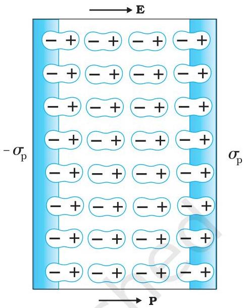FIGURE 2.23 A uniformly polarised dielectric amounts to induced surface charge density, but no volume charge density.

2.11 CAPACITORS AND CAPACITANCE

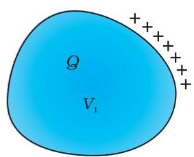
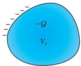
A capacitor is a system of two conductors separated by an insulator (Fig. 2.24). The conductors have charges, say $Q_{1}$ and $Q_{2}$, and potentials $V_{1}$ and $V_{2}$. Usually, in practice, the two conductors have charges $Q$ and $-Q$, with potential difference $V = V_{1} - V_{2}$ between them. We shall consider only this kind of charge configuration of the capacitor. (Even a single conductor can be used as a capacitor by assuming the other at infinity.) The conductors may be so charged by connecting them to the two terminals of a battery. $Q$ is called the charge of the capacitor, though this, in fact, is the charge on one of the conductors – the total charge of the capacitor is zero.

The electric field in the region between the conductors is proportional to the charge $Q$. That is, if the charge on the capacitor is, say doubled, the electric field will also be doubled at every point. (This follows from the direct proportionality between field and charge implied by Coulomb's law and the superposition principle.) Now, potential difference $V$ is the work done per unit positive charge in taking a small test charge from the conductor 2 to 1 against the field. Consequently, $V$ is also proportional to $Q$, and the ratio $Q / V$ is a constant:

$ C = \frac {Q}{V} \tag {2.38} $

The constant $C$ is called the capacitance of the capacitor. $C$ is independent of $Q$ or $V$, as stated above. The capacitance $C$ depends only on the

Conductor 1

Conductor 2 FIGURE 2.24 A system of two conductors separated by an insulator forms a capacitor.

geometrical configuration (shape, size, separation) of the system of two conductors. [As we shall see later, it also depends on the nature of the insulator (dielectric) separating the two conductors.] The SI unit of capacitance is 1 farad (=1 coulomb $\mathrm{volt}^{-1}$ ) or $1\mathrm{F} = 1\mathrm{C}\mathrm{V}^{-1}$ . A capacitor with fixed capacitance is symbolically shown as $-||-$,
while the one with variable capacitance is shown as $-|/|-$ with a diagonal arrow across it..

Equation (2.38) shows that for large $C$, $V$ is small for a given $Q$. This means a capacitor with large capacitance can hold large amount of charge $Q$ at a relatively small $V$. This is of practical importance. High potential difference implies strong electric field around the conductors. A strong electric field can ionise the surrounding air and accelerate the charges so produced to the oppositely charged plates, thereby neutralising the charge on the capacitor plates, at least partly. In other words, the charge of the capacitor leaks away due to the reduction in insulating power of the intervening medium.

The maximum electric field strength that a dielectric medium can sustain without undergoing electrical breakdown (i.e., losing its insulating properties) is termed its dielectric strength; for atmospheric air, this value is approximately $3 \times 10^{6} \mathrm{Vm}^{-1}$. When considering a separation of around $1 \mathrm{cm}$ between conductors, this electric field corresponds to a potential difference of $3 \times 10^{4} \mathrm{V}$ across them. Therefore, for a capacitor to effectively store a substantial amount of charge without premature discharge, its capacitance must be sufficiently high such that the resulting potential difference, and consequently the electric field, does not exceed these breakdown limits. Stated otherwise, there is an inherent upper bound to the quantity of charge that can be accumulated on a given capacitor without experiencing significant leakage. In practical applications, the farad is an exceptionally large unit; the most frequently encountered units are its sub-multiples, such as $1 \mu \mathrm{F} = 10^{-6} \mathrm{~F}$, $1 \mathrm{nF} = 10^{-9} \mathrm{F}$, $1 \mathrm{pF} = 10^{-12} \mathrm{F}$, and so forth. Beyond its primary function of charge storage, a capacitor constitutes a vital component in the majority of alternating current (AC) circuits, fulfilling critical roles as elaborated in Chapter 7.

2.12 THE PARALLEL PLATE CAPACITOR

A parallel plate capacitor is composed of two large, planar, conductive plates positioned in parallel, separated by a modest distance (Fig. 2.25). Initially, we consider the space between these plates to be a vacuum; the influence of a dielectric material will be addressed in a subsequent discussion. Let $A$ represent the surface area of each plate and $d$ denote their separation. The plates carry charges of $Q$ and $-Q$ respectively. Given that the separation $d$ is significantly smaller than the linear dimensions of the plates ($d^2 \ll A$), it is permissible to apply the principle for the electric field generated by an infinite plane sheet possessing a uniform surface charge density (refer to Section 1.15). Plate 1 exhibits a surface charge density of $\sigma = Q / A$, while plate 2 has a surface charge density of $-\sigma$. Employing Eq. (1.33), the electric field distribution across various regions is determined as follows:

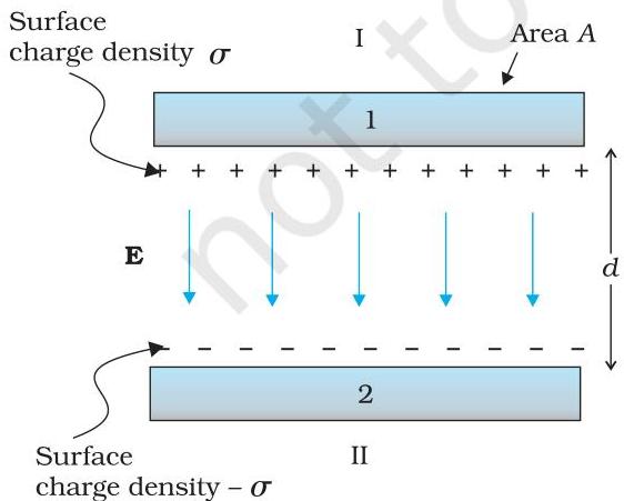FIGURE 2.25 The parallel plate capacitor.

For the outer region I (above plate 1),

$ E = \frac {\sigma}{2 \varepsilon_ {0}} - \frac {\sigma}{2 \varepsilon_ {0}} = 0 \tag {2.39} $

For the outer region II (below plate 2),

$ E = \frac {\sigma}{2 \varepsilon_ {0}} - \frac {\sigma}{2 \varepsilon_ {0}} = 0 \tag {2.40} $

In the interior region situated between plates 1 and 2, the electric fields originating from the two charged plates superpose, resulting in

$ E = \frac {\sigma}{2 \varepsilon_ {0}} + \frac {\sigma}{2 \varepsilon_ {0}} = \frac {\sigma}{\varepsilon_ {0}} = \frac {Q}{\varepsilon_ {0} A} \tag {2.41} $

The electric field vectors point from the positively charged plate towards the negatively charged plate.

Consequently, the electric field is confined to the space between the two plates and exhibits a uniform distribution throughout this region. However, for plates of finite extent, this uniformity does not hold true in the vicinity of their outer perimeters. The field lines curve outwards at the edges, a phenomenon known as 'field fringing'. Similarly, the surface charge density $\sigma$ will not be perfectly uniform across the entire plate. (Equation (2.35) establishes the relationship between $E$ and $\sigma$.) Nevertheless, under the condition $d^2 \ll A$, these edge effects can be disregarded in areas sufficiently distant from the boundaries, where the field remains accurately described by Eq. (2.41). Considering a uniform electric field, the potential difference is directly given by the product of the electric field strength and the separation between the plates, specifically:

$ V = E d = \frac {1}{\varepsilon_ {0}} \frac {Q d}{A} \tag {2.42} $

The capacitance $C$ for this parallel plate configuration is subsequently determined as:

$ C = \frac {Q}{V} = \frac {\varepsilon_ {0} A}{d} \tag {2.43} $

which, as anticipated, is solely dependent on the geometric properties of the system. Considering representative parameters, such as an area $A = 1 , \text{m}^2$ and a separation $d = 1 , \text{mm}$, the capacitance value obtained is:

$ C = \frac {8.85 \times 10^{-12} , \mathrm{C}^2 , \mathrm{N}^{-1} , \mathrm{m}^{-2} \times 1 , \mathrm{m}^2}{10^{-3} , \mathrm{m}} = 8.85 \times 10^{-9} , \mathrm{F} \tag {2.44} $

(It can be verified that $1 , \mathrm{F} = 1 , \mathrm{C} , \mathrm{V}^{-1} = 1 , \mathrm{C} , (\mathrm{NC}^{-1} , \mathrm{m})^{-1} = 1 , \mathrm{C}^2 , \mathrm{N}^{-1} , \mathrm{m}^{-1}$.) This calculation underscores that $1 , \mathrm{F}$ represents a unit of considerable magnitude for practical applications, as previously noted. An alternative perspective to appreciate the substantial size of $1 , \mathrm{F}$ involves determining the plate area required to achieve $C = 1 , \mathrm{F}$ with a plate separation of, for instance, $1 , \mathrm{cm}$:

$ A = \frac {C d}{\varepsilon_ {0}} = \frac {1 , \mathrm{F} \times 10^{-2} , \mathrm{m}}{8.85 \times 10^{-12} , \mathrm{C}^2 , \mathrm{N}^{-1} , \mathrm{m}^{-2}} = 10^{9} , \mathrm{m}^2 \tag {2.45} $

which is a plate about $30 , \mathrm{km}$ in length and breadth!

2.13 EFFECT OF DIELECTRIC ON CAPACITANCE

Building upon the insights into dielectric behavior within an external electric field, as detailed in Section 2.10, we now examine how the capacitance of a parallel plate capacitor undergoes alteration when a dielectric material is introduced. Our configuration remains a pair of expansive plates, each possessing area $A$, separated by a distance $d$. These plates carry charges of $\pm Q$, which corresponds to a surface charge density of $\pm \sigma$ (where $\sigma = Q / A$). In the scenario where a vacuum occupies the space between the plates,

$ E _ {0} = \frac {\sigma}{\varepsilon_ {0}} $

and the resultant potential difference, denoted $V_{0}$, is given by

$ V _ {0} = E _ {0} d $

The capacitance $C_0$ for this vacuum configuration is consequently

$ C _ {0} = \frac {Q}{V _ {0}} = \varepsilon_ {0} \frac {A}{d} \tag {2.46} $

Now, let us consider a dielectric material completely filling the space between these plates. The presence of the electric field induces polarization within the dielectric. As elaborated in Section 2.10, this polarization manifests as an effective pair of charged sheets positioned at the dielectric's surfaces perpendicular to the field, bearing surface charge densities of $\sigma_{p}$ and $-\sigma_{p}$. Consequently, the electric field within the dielectric can be understood as arising from a net surface charge density on the plates equal to $\pm (\sigma - \sigma_{p})$. Specifically,

$ E = \frac {\sigma - \sigma_ {P}}{\varepsilon_ {0}} \tag {2.47} $

thereby establishing a potential difference $V$ across the plates as

$ V = E d = \frac {\sigma - \sigma_ {P}}{\varepsilon_ {0}} d \tag {2.48} $

In the context of linear dielectrics, it is anticipated that $\sigma_{p}$ will exhibit proportionality to $E_0$, and by extension, to $\sigma$. This implies that the term $(\sigma - \sigma_{p})$ is also directly proportional to $\sigma$, allowing us to express this relationship as:

$ \sigma - \sigma_ {P} = \frac {\sigma}{K} \tag {2.49} $

where $K$ represents a constant intrinsic to the dielectric material. It is evident that $K > 1$. This leads to the following expression for

the potential

difference:

$

V = \frac {\sigma d}{\varepsilon_ {0} K} = \frac {Q d}{A \varepsilon_ {0} K} \tag {2.50} $

Consequently, the capacitance $C$, when the dielectric fully occupies the space between the plates, is determined as

$ C = \frac {Q}{V} = \frac {\varepsilon_ {0} K A}{d} \tag {2.51} $

The quantity $\varepsilon_0 K$ is defined as the permittivity of the medium and is symbolized by $\varepsilon$

$ \varepsilon = \varepsilon_ {0} K \tag {2.52} $

In the case of a vacuum, $K=1$, which implies $\varepsilon = \varepsilon_0$; here, $\varepsilon_0$ is designated as the permittivity of free space. The dimensionless quotient

$ K = \frac {\varepsilon}{\varepsilon_ {0}} \tag {2.53} $

is termed the dielectric constant of the material. As previously noted, deriving from Eq. (2.49), it is evident that $K$ must be greater than 1. By comparing Eq. (2.46) and Eq. (2.51),

$ K = \frac {C}{C _ {0}} \tag {2.54} $

Consequently, the dielectric constant of a material quantifies the factor (which is greater than 1) by which the capacitance is augmented from its value in vacuum, provided the dielectric completely fills the space between a capacitor's plates. Although this derivation was initiated by considering

Eq. (2.54) for the case of a parallel plate capacitor, it holds good for any type of capacitor and can, in fact, be viewed in general as a definition of the dielectric constant of a substance.

Example 2.8 A slab of material of dielectric constant $K$ has the same area as the plates of a parallel-plate capacitor but has a thickness $(3/4)d$, where $d$ is the separation of the plates. How is the capacitance changed when the slab is inserted between the plates?

Solution Let $E_0 = V_0 / d$ be the electric field between the plates when there is no dielectric and the potential difference is $V_0$. If the dielectric is now inserted, the electric field in the dielectric will be $E = E_0 / K$. The potential difference will then be

$ \begin{array}{l} V = E_0 \left(\frac{1}{4} d\right) + \frac{E_0}{K} \left(\frac{3}{4} d\right) \ = E_0 d \left(\frac{1}{4} + \frac{3}{4K}\right) = V_0 \frac{K + 3}{4K} \end{array} $

The potential difference decreases by the factor $(K + 3) / 4K$ while the free charge $Q_0$ on the plates remains unchanged. The capacitance thus increases

$ C = \frac{Q_0}{V} = \frac{4K}{K + 3} \frac{Q_0}{V_0} = \frac{4K}{K + 3} C_0 $

2.14 COMBINATION OF CAPACITORS

We can combine several capacitors of capacitance $C_1, C_2, \ldots, C_n$ to obtain a system with some effective capacitance $C$. The effective capacitance depends on the way the individual capacitors are combined. Two simple possibilities are discussed below.

2.14.1 Capacitors in series

Figure 2.26 shows capacitors $C_1$ and $C_2$ combined in series.

The left plate of $C_1$ and the right plate of $C_2$ are connected to two terminals of a battery and have charges $Q$ and $-Q$, respectively. It then follows that the right plate of $C_1$ has charge $-Q$ and the left plate of $C_2$ has charge $Q$. If this was not so, the net charge on each capacitor would not be zero. This would result in an electric field in the conductor connecting $C_1$ and $C_2$. Charge would flow until the net charge on both $C_1$ and $C_2$ is zero and there is no electric field in the conductor connecting $C_1$ and $C_2$. Thus, in the series combination, charges on the two plates $(\pm Q)$ are the same on each capacitor. The total

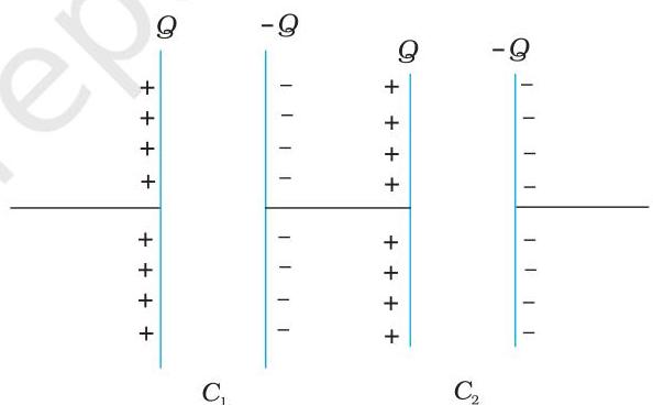FIGURE 2.26 Combination of two capacitors in series.

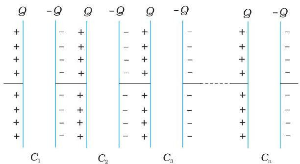FIGURE 2.27 Combination of n capacitors in series.

potential drop $V$ across the combination is the sum of the potential drops $V_{1}$ and $V_{2}$ across $C_1$ and $C_2$, respectively.

$ V = V _ {1} + V _ {2} = \frac {Q}{C _ {1}} + \frac {Q}{C _ {2}} \tag {2.55} $

$ \text{i.e.,} \frac {V}{Q} = \frac {1}{C _ {1}} + \frac {1}{C _ {2}}, \tag {2.56} $

Now we can regard the combination as an effective capacitor with charge $Q$ and potential difference $V$. The effective capacitance of the combination is

$ C = \frac {Q}{V} \tag {2.57} $

We compare Eq. (2.57) with Eq. (2.56), and obtain

$ \frac {1}{C} = \frac {1}{C _ {1}} + \frac {1}{C _ {2}} \tag {2.58} $

The proof clearly goes through for any number of capacitors arranged in a similar way. Equation (2.55), for $n$ capacitors arranged in series, generalises to

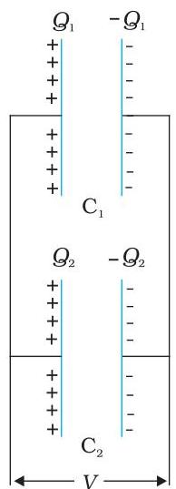(a)

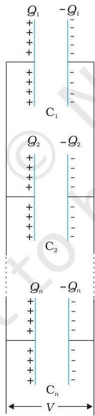(b) FIGURE 2.28 Parallel combination of (a) two capacitors, (b) n capacitors.

$ V = V _ {1} + V _ {2} + \dots + V _ {n} = \frac {Q}{C _ {1}} + \frac {Q}{C _ {2}} + \dots + \frac {Q}{C _ {n}} \tag {2.59} $

Following the same steps as for the case of two capacitors, we get the general formula for effective capacitance of a series combination of $n$ capacitors:

$ \frac {1}{C} = \frac {1}{C _ {1}} + \frac {1}{C _ {2}} + \frac {1}{C _ {3}} + \dots + \frac {1}{C _ {n}} \tag {2.60} $

2.14.2 Capacitors in parallel

Figure 2.28 (a) shows two capacitors arranged in parallel. In this case, the same potential difference is applied across both the capacitors. But the plate charges $(\pm Q_{1})$ on capacitor 1 and the plate charges $(\pm Q_{2})$ on the capacitor 2 are not necessarily the same:

$ Q _ {1} = C _ {1} V, Q _ {2} = C _ {2} V \tag {2.61} $

The equivalent capacitor is one with charge

$ Q = Q _ {1} + Q _ {2} \tag {2.62} $

and potential difference $V$.

$ Q = C V = C _ {1} V + C _ {2} V \tag {2.63} $

The effective capacitance C is, from Eq. (2.63),

$ C = C _ {1} + C _ {2} \tag {2.64} $

The general formula for effective capacitance $C$ for parallel combination of $n$ capacitors [Fig. 2.28 (b)] follows similarly,

$ Q = Q _ {1} + Q _ {2} + \dots + Q _ {n} \tag {2.65} $

$ \text{i.e., } C V = C _ {1} V + C _ {2} V + \dots C _ {n} V \tag {2.66} $

which gives

$ C = C _ {1} + C _ {2} + \dots C _ {n} \tag {2.67} $

Example 2.9 A network of four $10~\mu \mathrm{F}$ capacitors is connected to a $500\mathrm{V}$ supply, as shown in Fig. 2.29. Determine (a) the equivalent capacitance of the network and (b) the charge on each capacitor. (Note, the charge on a capacitor is the charge on the plate with higher potential, equal and opposite to the charge on the plate with lower potential.)

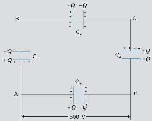FIGURE 2.29

Solution

(a) In the given network, $C_1$, $C_2$ and $C_3$ are connected in series. The effective capacitance $C'$ of these three capacitors is given by

$ \frac {1}{C ^ {\prime}} = \frac {1}{C _ {1}} + \frac {1}{C _ {2}} + \frac {1}{C _ {3}} $

For $C_1 = C_2 = C_3 = 10 \mu \mathrm{F}$, $C' = (10/3) \mu \mathrm{F}$. The network has $C'$ and $C_4$ connected in parallel. Thus, the equivalent capacitance $C$ of the network is

$ C = C ^ {\prime} + C _ {4} = \left(\frac {1 0}{3} + 1 0\right) \mu \mathrm {F} = 1 3. 3 \mu \mathrm {F} $

(b) Clearly, from the figure, the charge on each of the capacitors, $C_1$, $C_2$ and $C_3$ is the same, say $Q$. Let the charge on $C_4$ be $Q'$. Now, since the potential difference across AB is $Q / C_1$, across BC is $Q / C_2$, across CD is $Q / C_3$, we have

$ \frac {Q}{C _ {1}} + \frac {Q}{C _ {2}} + \frac {Q}{C _ {3}} = 5 0 0 \mathrm {V}, $

Also, $ Q^{\prime} / C_{4} = 500\mathrm{V} $

This gives for the given value of the capacitances,

$ Q =