Chapter Four
MOVING CHARGES AND MAGNETISM
4.1 INTRODUCTION
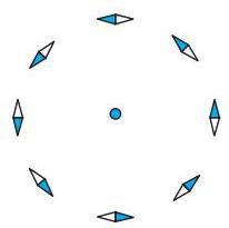
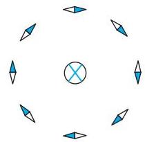
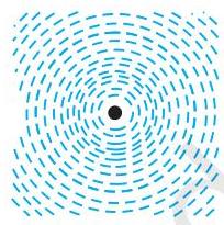
For over two millennia, the distinct phenomena of electricity and magnetism were recognized. Yet, it was not until approximately two centuries ago, specifically in 1820, that their fundamental interconnectedness became apparent. In the summer of that year, during a public demonstration, the Danish physicist Hans Christian Oersted observed that an electric current flowing through a straight conductor produced a discernible deflection in a magnetic compass needle positioned nearby. His subsequent investigations revealed that the compass needle's orientation consistently aligned tangentially to a hypothetical circular path centered on the straight wire, with its plane orthogonal to the wire itself, as illustrated in Fig. 4.1(a). This effect was particularly prominent when the current was substantial and the compass needle was sufficiently proximate to the conductor, thereby minimizing the influence of Earth's magnetic field. A reversal in the current's direction correspondingly inverted the needle's alignment [Fig. 4.1(b)]. Furthermore, the magnitude of the deflection intensified with either an increase in the current or a reduction in the distance between the needle and the wire. When iron filings were scattered around the wire, they coalesced into concentric circular patterns with the wire at their nucleus [Fig. 4.1(c)]. From these observations, Oersted deduced that moving electrical charges, or currents, generate a magnetic field within their vicinity.
Oersted's discovery spurred a period of vigorous experimental inquiry. By 1864,
James Maxwell successfully synthesized and articulated the governing principles of electricity and magnetism, subsequently recognizing light as a form of electromagnetic radiation. Towards the close of the $19^{\text{th}}$ century, radio waves were identified by Hertz and successfully generated by J.C. Bose and G. Marconi. The $20^{\text{th}}$ century witnessed profound scientific and technological advancements, largely attributable to an enhanced comprehension of electromagnetism and the development of apparatuses for the generation, amplification, transmission, and detection of electromagnetic waves.
 (a)
(a)
 (b)
(b)
 (c)
FIGURE 4.1 The magnetic field due to a straight long current-carrying wire. The wire is perpendicular to the plane of the paper. A ring of compass needles surrounds the wire. The orientation of the needles is shown when (a) the current emerges out of the plane of the paper, (b) the current moves into the plane of the paper. (c) The arrangement of iron filings around the wire. The darkened ends of the needle represent north poles. The effect of the earth's magnetic field is neglected.
(c)
FIGURE 4.1 The magnetic field due to a straight long current-carrying wire. The wire is perpendicular to the plane of the paper. A ring of compass needles surrounds the wire. The orientation of the needles is shown when (a) the current emerges out of the plane of the paper, (b) the current moves into the plane of the paper. (c) The arrangement of iron filings around the wire. The darkened ends of the needle represent north poles. The effect of the earth's magnetic field is neglected.
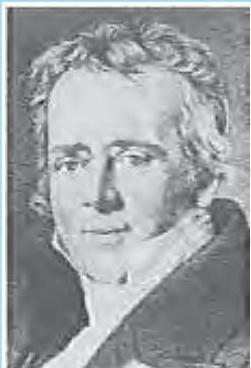
Hans Christian Oersted (1777-1851), a Danish physicist and chemist who held a professorship at Copenhagen, observed that a compass needle would deviate when positioned close to a conductor through which an electric current flowed. This pivotal finding furnished the initial empirical proof of an intrinsic link between electrical and magnetic phenomena.
This chapter delves into the forces exerted by magnetic fields on moving charged entities, including electrons, protons, and current-carrying conductors. We will also ascertain how electric currents generate magnetic fields. Additionally, the mechanisms enabling particle acceleration to very high energies within a cyclotron will be discussed, alongside the operation of galvanometers for current and voltage detection.
For the present and subsequent chapters concerning magnetism, a specific convention is employed: a current or a field (whether electric or magnetic) directed outward from the plane of observation is represented by a dot $\odot$ Conversely, a current or field entering the plane of observation is denoted by a cross $(\otimes)^{*}$. These two scenarios are illustrated in Figures 4.1(a) and 4.1(b), respectively.
4.2 MAGNETIC FORCE
4.2.1 Sources and fields
Prior to introducing the magnetic field $\mathbf{B}$, it is beneficial to review the fundamental aspects of the electric field $\mathbf{E}$ covered in Chapter 1. The interaction between any two charges is conceptually understood as a two-stage process: initially, a source charge $\mathbf{Q}$ establishes an electric field $\mathbf{E}$, defined as:
$ \mathbf {E} = Q \hat {\mathbf {r}} / \left(4 \pi \varepsilon_ {0}\right) r ^ {2} \tag {4.1} $
Here, $\hat{\mathbf{r}}$ denotes the unit vector oriented along $\mathbf{r}$, and $\mathbf{E}$ itself constitutes a vector field. Subsequently, a charge $q$ positioned within this field will interact with it, experiencing a force $\mathbf{F}$ quantified as:
$ \mathbf {F} = q \mathbf {E} = q Q \hat {\mathbf {r}} / \left(4 \pi \varepsilon_ {0}\right) r ^ {2} \tag {4.2} $
As previously established in Chapter 1, the electric field $\mathbf{E}$ transcends a mere mathematical construct, possessing a tangible physical reality. It is capable of transmitting both energy and momentum, and its establishment is not instantaneous but requires a finite propagation time. The profound significance of the field concept was particularly emphasized by Faraday and subsequently integrated by Maxwell into his comprehensive unification of electricity and magnetism. While an electric field can inherently vary with time, thereby functioning as a time-dependent entity, for the purposes of the current chapter's discourse, we shall proceed under the assumption that these fields remain static.
The resultant field at any given spatial point may originate from a single charge or a multiplicity of charges. In instances involving multiple charges, their individual fields combine through vector addition. This fundamental concept, known as the principle of superposition, was introduced in Chapter 1. With the electric field thus determined, the force exerted upon a test charge can be calculated using Equation (4.2).
Analogous to the generation of an electric field by static charges, electric currents or charges in motion concurrently establish a magnetic field, designated as $\mathbf{B}(\mathbf{r})$. This magnetic field also functions as a vector field and exhibits several fundamental characteristics shared with the electric field. It is spatially defined at every point (and can similarly possess time dependence). Empirical observations confirm that the magnetic field adheres to the principle of superposition; specifically, the total magnetic field arising from multiple sources is the vector sum of the magnetic fields produced by each source independently.
4.2.2 Magnetic Field, Lorentz Force
Consider a point charge, denoted by $q$, situated at position $\mathbf{r}$ at time $t$ and possessing a velocity $\mathbf{v}$. When this charge is subjected to both an electric field $\mathbf{E}(\mathbf{r})$ and a magnetic field $\mathbf{B}(\mathbf{r})$, the cumulative force exerted upon it is expressed as:
$ \mathbf {F} = q \left[ \mathbf {E} (\mathbf {r}) + \mathbf {v} \times \mathbf {B} (\mathbf {r}) \right] \equiv \mathbf {F} _ {\text {electric}} + \mathbf {F} _ {\text {magnetic}} \tag {4.3} $
This fundamental force relationship, known as the Lorentz force, was initially formulated by H.A. Lorentz, drawing upon the comprehensive experimental findings of scientists like Ampere. While the force originating from an electric field has been thoroughly examined previously, the interaction specifically involving the magnetic field exhibits distinct characteristics, which are outlined below.
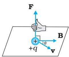
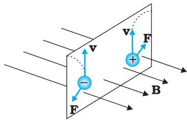
(i) The magnetic force is contingent upon the particle's charge ($q$), its velocity ($\mathbf{v}$), and the strength and direction of the magnetic field ($\mathbf{B}$). Notably, a negatively charged particle experiences a magnetic force in the direction precisely contrary to that experienced by a positively charged particle under identical conditions. (ii) The magnetic force, expressed as $q[\mathbf{v} \times \mathbf{B}]$, inherently involves a vector cross product between the velocity vector and the magnetic field vector. A direct consequence of this vector product is that the magnetic force becomes null (zero) when the velocity and magnetic field vectors are either parallel or anti-parallel. The resultant force is invariably directed perpendicularly to both the velocity vector and the magnetic field vector. Its precise orientation is determined by either the screw rule or the right-hand rule, commonly employed for vector (or cross) products, as depicted in Fig. 4.2.
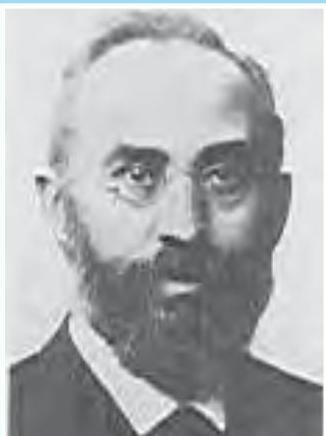
Hendrik Antoon Lorentz (1853 - 1928) was a Dutch theoretical physicist and a professor at Leiden University. His research focused on the interrelationships among electricity, magnetism, and mechanics. To elucidate the observed influence of magnetic fields on light emitters (known as the Zeeman effect), he posited the existence of electric charges within the atom, an achievement for which he was awarded the Nobel Prize in 1902. He also formulated a set of transformation equations, subsequently named after him as the Lorentz transformation equations, through intricate mathematical reasoning, though he did not fully recognize at the time that these equations were fundamentally rooted in novel concepts of space and time.
 (a)
(a)
 (b)
FIGURE 4.2 The direction of the magnetic force acting on a charged particle. (a) The force on a positively charged particle with velocity $\mathbf{v}$ and making an angle $\theta$ with the magnetic field $\mathbf{B}$ is given by the right-hand rule. (b) A moving charged particle $q$ is deflected in an opposite sense to $-q$ in the presence of magnetic field.
(b)
FIGURE 4.2 The direction of the magnetic force acting on a charged particle. (a) The force on a positively charged particle with velocity $\mathbf{v}$ and making an angle $\theta$ with the magnetic field $\mathbf{B}$ is given by the right-hand rule. (b) A moving charged particle $q$ is deflected in an opposite sense to $-q$ in the presence of magnetic field.
(iii) Should the charge be stationary, i.e., $|\mathbf{v}| = 0$, the magnetic force exerted upon it is identically zero. Consequently, only charges in motion experience a magnetic force.
The mathematical formulation of the magnetic force provides a basis for defining the standard unit of the magnetic field. This definition arises by considering the force equation $\mathbf{F} = q[\mathbf{v} \times \mathbf{B}] = qvB\sin \theta \hat{\mathbf{n}}$, where $\theta$ represents the angle between $\mathbf{v}$ and $\mathbf{B}$ (refer to Fig. 4.2 (a)). If $q$, $\mathbf{F}$, and $\mathbf{v}$ are all set to unity, the magnitude of the magnetic field $B$ is defined as 1 SI unit under specific conditions: when a force of one newton acts upon a unit charge (1 Coulomb) moving at a speed of 1 m/s perpendicularly to the magnetic field $\mathbf{B}$.
Dimensionally, we have $[B] = [F / qv]$ and the unit of $\mathbf{B}$ are Newton second / (coulomb metre). This unit is called tesla (T) named after Nikola Tesla (1856 - 1943). Tesla is a rather large unit. A smaller unit (non-SI) called gauss ( $= 10^{-4}$ tesla) is also often used. The earth's magnetic field is about $3.6 \times 10^{-5}$ T.
4.2.3 Magnetic force on a current-carrying conductor
We can extend the analysis for force due to magnetic field on a single moving charge to a straight rod carrying current. Consider a rod of a uniform cross-sectional area $A$ and length $l$. We shall assume one kind of mobile carriers as in a conductor (here electrons). Let the number density of these mobile charge carriers in it be $n$. Then the total number of mobile charge carriers in it is $nlA$. For a steady current $I$ in this conducting rod, we may assume that each mobile carrier has an average drift velocity $\mathbf{v}_{d}$ (see Chapter 3). In the presence of an external magnetic field $\mathbf{B}$, the force on these carriers is:
$ \mathbf {F} = (n l A) q \mathbf {v} _ {d} \times \mathbf {B} $
where $q$ is the value of the charge on a carrier. Now $nq\mathbf{v}{\mathrm{d}}$ is the current density $\mathbf{j}$ and $|(nq\mathbf{v}{\mathrm{d}})|A$ is the current $I$ (see Chapter 3 for the discussion of current and current density). Thus,
$ \begin{array}{l} \mathbf {F} = \left[ \left(n q \mathbf {v} _ {d}\right) l A \right] \times \mathbf {B} = [ \mathbf {j} A l ] \times \mathbf {B} \ = I \boldsymbol {l} \times \mathbf {B} \tag {4.4} \ \end{array} $
where $l$ is a vector of magnitude $l$, the length of the rod, and with a direction identical to the current $I$. Note that the current $I$ is not a vector. In the last step leading to Eq. (4.4), we have transferred the vector sign from $j$ to $l$.
Equation (4.4) holds for a straight rod. In this equation, $\mathbf{B}$ is the external magnetic field. It is not the field produced by the current-carrying rod. If the wire has an arbitrary shape we can calculate the Lorentz force on it by considering it as a collection of linear strips $\mathrm{d}l_{\mathrm{j}}$ and summing
$ \mathbf {F} = \sum_ {j} \operatorname {I d} l _ {j} \times \mathbf {B} $
This summation can be converted to an integral in most cases.
Example 4.1 A straight wire of mass $200\mathrm{g}$ and length $1.5\mathrm{m}$ carries a current of 2 A. It is suspended in mid-air by a uniform horizontal magnetic field $\mathbf{B}$ (Fig. 4.3). What is the magnitude of the magnetic field?
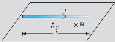 FIGURE 4.3
Solution From Eq. (4.4), we find that there is an upward force $\mathbf{F}$, of magnitude $IlB$. For mid-air suspension, this must be balanced by the force due to gravity:
$ m g = I l B $
$ \begin{array}{l} B = \frac {m g}{I l} \ = \frac {0 . 2 \times 9 . 8}{2 \times 1 . 5} = 0. 6 5 \mathrm {T} \ \end{array} $
It would have been adequate to provide $\mathrm{m} / \mathrm{l}$, representing the wire's linear mass density. The Earth's magnetic field, roughly $4 \times 10^{-5}$ T, has been disregarded in this context.
Example 4.2 If the magnetic field is oriented parallel to the positive $y$-axis and a charged particle traverses along the positive $x$-axis (Fig. 4.4), determine the direction of the Lorentz force for (a) an electron (negative charge), and (b) a proton (positive charge).
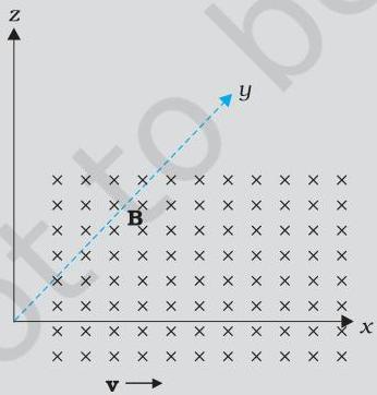 FIGURE 4.4
Solution: Given that the particle's velocity $\mathbf{v}$ is directed along the $x$-axis and the magnetic field $\mathbf{B}$ is aligned with the $y$-axis, the cross product $\mathbf{v} \times \mathbf{B}$ will point along the $z$-axis, as derived from the screw rule or right-hand thumb rule. Consequently, (a) for an electron, the force will be along the $-z$ axis, and (b) for a positive charge (proton), the force will be along the $+z$ axis.
4.3 MOTION IN A MAGNETIC FIELD
We shall now examine the behavior of a charge traversing a magnetic field with increased scrutiny. As established in Mechanics (refer to Chapter 5 of the Class XI textbook), work is performed by a force acting on a particle only if that force possesses a component aligned with (or opposing) the particle's direction of motion. However, for a charge moving within a magnetic field, the magnetic force consistently acts perpendicularly to the particle's velocity. This orthogonality implies that no work is done by the magnetic field, and thus, the kinetic energy (and consequently, the magnitude of the velocity) of the particle remains unaltered, although its momentum's direction may undergo modification. [It is important to note that this differs from the behavior of an electric field force, $q\mathbf{E}$, which can have a component parallel (or antiparallel) to the motion, thereby enabling both energy and momentum transfer.]
Our focus will be on the movement of a charged particle within a uniform magnetic field. Initially, let us analyze the scenario where the velocity $\mathbf{v}$ is orthogonal to the magnetic field $\mathbf{B}$. In this configuration, the magnetic force, represented by $q\mathbf{v} \times \mathbf{B}$, which is inherently perpendicular to both $\mathbf{v}$ and $\mathbf{B}$, functions as a centripetal force. This results in the particle executing circular motion within a plane perpendicular to the magnetic field. A particle will trace a circular path precisely when its velocity $\mathbf{v}$ and the magnetic field $\mathbf{B}$ are mutually perpendicular (Fig. 4.5).
Should the velocity possess a component parallel to $\mathbf{B}$, this longitudinal component will persist without alteration, given that motion along the magnetic field lines is unaffected by the field itself. Concurrently, the transverse motion, occurring in the plane perpendicular to $\mathbf{B}$, continues to be circular, as previously described. The combination of these two motions thus generates a helical trajectory (Fig. 4.6).
From prior studies (refer to Class XI, Chapter 3), it is known that for a particle traversing a circular path of radius $r$, a force of magnitude $m v^2 / r$ acts perpendicularly to its trajectory, directed towards the circle's center; this is termed the centripetal force. When the velocity $\mathbf{v}$ is perpendicular to the magnetic field $\mathbf{B}$, the resulting magnetic force is orthogonal to both $\mathbf{v}$ and $\mathbf{B}$, effectively serving as the centripetal force. Its magnitude is given by $q v B$. By equating these two formulations for the centripetal force,
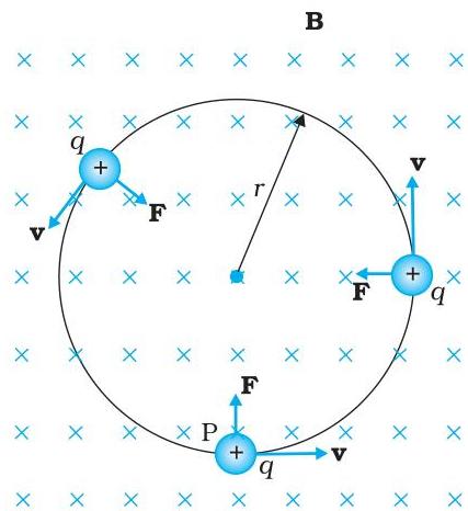 FIGURE 4.5 Circular motion
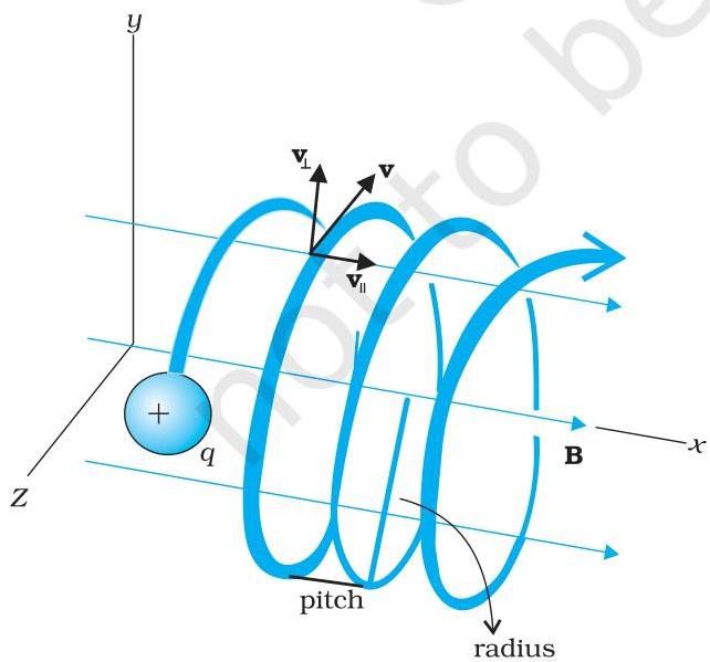 FIGURE 4.6 Helical motion
Equating the centripetal force to the magnetic Lorentz force, $m v^{2} / r = q v B$, yields the following expression for the radius:
$ r = m v / q B \tag {4.5} $
This expression defines the radius of the circular trajectory followed by the charged particle. A direct proportionality exists between the particle's momentum and the radius of its circular path; consequently, greater momentum corresponds to a larger trajectory. Considering $\omega$ as the angular frequency, the relationship $\nu = \omega r$ leads to:
$ \omega = 2 \pi \nu = q B / m \tag {4.6(a)} $
This result demonstrates that the frequency of rotation is invariant with respect to the particle's velocity or kinetic energy. The variable $\nu$ denotes the rotational frequency. This intrinsic independence of frequency from energy is a fundamental principle utilized in the engineering of cyclotrons.
The period required for a single revolution is given by $T = 2\pi / \omega \equiv 1 / \nu$. Should a velocity component exist parallel to the magnetic field (designated as $v_{||}$), it will induce motion of the particle along the field lines, resulting in a helical trajectory (Fig. 4.6). The axial displacement along the magnetic field during one complete rotation is termed the pitch, denoted by $p$. By employing Equation [4.6
(a)], the pitch can be expressed as:
$ p = v _ {0} T = 2 \pi m v _ {0} / q B \tag {4.6(b)} $
The radius of the circular trajectory within this helical motion is referred to as the helix radius.
Example 4.3 Determine the trajectory radius for an electron (possessing a mass of $9 \times 10^{-31} \mathrm{kg}$ and a charge of $1.6 \times 10^{-19} \mathrm{C}$) traversing a magnetic field of $6 \times 10^{-4} \mathrm{T}$ at a speed of $3 \times 10^{7} \mathrm{m/s}$, where the velocity is perpendicular to the field. Additionally, ascertain its frequency and compute its energy in kiloelectron volts (given $1 \mathrm{eV} = 1.6 \times 10^{-19} \mathrm{J}$).
Solution: Applying Equation (4.5), we compute:
$ \begin{array}{l} r = m v / (q B) = 9 \times 10^{-31} \mathrm {k g} \times 3 \times 10^{7} \mathrm {m s} ^ {- 1} / (1.6 \times 10^{-19} \mathrm {C} \times 6 \times 10^{-4} \mathrm {T}) \ = 28 \times 10^{-2} \mathrm {m} = 28 \mathrm {c m} \ \end{array} $
$ \begin{array}{l} \nu = v / (2 \pi r) = 17 \times 10^{6} \mathrm {s} ^ {- 1} = 17 \times 10^{6} \mathrm {H z} = 17 \mathrm {M H z}. \ E = \left(\frac {1}{2}\right) m v ^ {2} = \left(\frac {1}{2}\right) 9 \times 10^{-31} \mathrm {k g} \times 9 \times 10^{14} \mathrm {m} ^ {2} / \mathrm {s} ^ {2} = 40.5 \times 10^{-17} \mathrm {J} \ \approx 4 \times 10^{-16} \mathrm {J} = 2.5 \mathrm {k e V}. \ \end{array} $
4.4 MAGNETIC FIELD DUE TO A CURRENT ELEMENT, BIOT-SAVART LAW
The entirety of observed magnetic fields originates from either electric currents (or charges in motion) or the inherent magnetic moments of fundamental particles. Our focus here will be on elucidating the connection between an electric current and the magnetic field it generates, a relationship defined by Biot-Savart's law. As depicted in Fig. 4.7, consider a conductor segment XY carrying a current $I$. To analyze the magnetic field, we isolate an infinitesimal element $\mathrm{d}l$ within this conductor. The objective is to determine the magnetic field $\mathrm{dB}$ produced by this specific element at a point $P$, located at a radial distance $r$ from it. The angle between the current element vector $\mathrm{d}\mathbf{l}$ and the displacement vector $\mathbf{r}$ is denoted by $\theta$. Biot-Savart's law postulates that the magnitude of the magnetic field $\mathrm{dB}$ is directly proportional to the current $I$, the scalar length of the element $|\mathrm{d}\mathbf{l}|$, and inversely proportional to the square of the distance $r$. Furthermore, its direction* is orthogonal to the plane established by $\mathrm{d}\mathbf{l}$ and $\mathbf{r}$. Consequently, in its vector formulation,
$ \begin{array}{l} d \mathbf {B} \propto \frac {I d \mathbf {l} \times \mathbf {r}}{r ^ {3}} \ = \frac {\mu_ {0}}{4 \pi} \frac {I d \mathbf {l} \times \mathbf {r}}{r ^ {3}} \tag {4.7(a)} \ \end{array} $
Here, $\mu_0 / 4\pi$ serves as the proportionality constant. This particular formulation is valid under the condition that the surrounding medium is a vacuum.
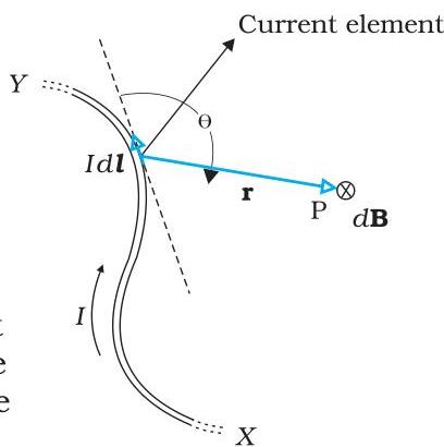 FIGURE 4.7 Depiction of the Biot-Savart law. The current element $I , \mathrm{d}l$ generates a magnetic field $\mathrm{dB}$ at a radial separation $r$. The symbol $\otimes$ signifies that the magnetic field vector is oriented perpendicularly into the plane of the page.
The scalar magnitude of this magnetic field is expressed as:
$ \left| \mathrm {d} \mathbf {B} \right| = \frac {\mu_ {0}}{4 \pi} \frac {I \mathrm {d} l \sin \theta}{r ^ {2}} \tag {4.7(b)} $
This form is derived by applying the properties of the vector cross-product. Equation [4.7 (a)] serves as the fundamental relationship for calculating the magnetic field. In SI units, the proportionality constant possesses the precise value:
$ \frac {\mu_ {0}}{4 \pi} = 1 0 ^ {- 7} \mathrm {T m / A} \tag {4.7(c)} $
The term $\mu_0$ is designated as the permeability of free space (or vacuum).
The Biot-Savart law, which describes the magnetic field, exhibits both parallels and distinctions when compared to Coulomb's law, which governs the electrostatic field. These include:
(i) Both phenomena are long-range interactions, characterized by an inverse square dependence on the distance separating the source from the observation point. Furthermore, the principle of superposition is applicable to both field types. [It is pertinent to note here that the magnetic field demonstrates linearity with respect to its source, $I\mathrm{d}l$, analogous to how the electrostatic field is linear with its source, the electric charge.] (ii) The electrostatic field originates from a scalar source, specifically electric charge. In contrast, the magnetic field is generated by a vector source, represented by $I , \mathrm{d}l$. (iii) The electrostatic field vector is collinear with the displacement vector connecting the source and the field point. Conversely, the magnetic field vector is orthogonal to the plane defined by the displacement vector $\mathbf{r}$ and the current element $I\mathrm{d}\mathbf{l}$. (iv) A notable characteristic of the Biot-Savart law, absent in the electrostatic context, is its dependence on the angle. Referring to Fig. 4.7, the magnetic field vanishes at any point situated along the axis defined by $\mathrm{d}l$ (indicated by the dashed line). In this specific orientation, $\theta = 0$, which implies $\sin \theta = 0$, and consequently, from Eq. [4.7(a)], $|\mathrm{dB}| = 0$.
A notable relationship exists among $\varepsilon_0$, representing the permittivity of free space; $\mu_0$, denoting the permeability of free space; and $c$, the speed of light in a vacuum:
$ \varepsilon_ {0} \mu_ {0} = \left(4 \pi \varepsilon_ {0}\right) \frac {\mu_ {0}}{4 \pi} = \frac {1}{9 \times 1 0 ^ {9}} \left(1 0 ^ {- 7}\right) = \frac {1}{(3 \times 1 0 ^ {8}) ^ {2}} = \frac {1}{c ^ {2}} $
This interrelationship will be explored in greater detail within Chapter 8, which focuses on electromagnetic waves. Given that the speed of light in a vacuum is invariant, the product $\mu_0\varepsilon_0$ possesses a constant magnitude. Consequently, establishing the value for either $\varepsilon_0$ or $\mu_0$ inherently determines the value of the other. Within the International System of Units (SI), $\mu_0$ is precisely defined as $4\pi \times 10^{-7}$ in magnitude.
Example 4.4 A differential current element, $\Delta l = \Delta x\hat{i}$, is positioned at the coordinate origin, through which a significant current of $I = 10\mathrm{A}$ flows (refer to Fig. 4.8). Determine the magnetic field strength along the $y$-axis at a point $0.5\mathrm{m}$ away from the origin, given that $\Delta x = 1\mathrm{cm}$.
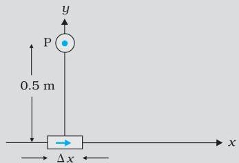 FIGURE 4.8
Solution
$ \left| \mathrm {d} \mathbf {B} \right| = \frac {\mu_ {0}}{4 \pi} \frac {I \mathrm {d} l \sin \theta}{r ^ {2}} [ \text {using Eq. (4.7)} ] $
$ \mathrm{d}l = \Delta x = 10^{-2} \mathrm{m}, I = 10 \mathrm{A}, r = 0.5 \mathrm{m} = y, \mu_0 / 4\pi = 10^{-7} \frac{\mathrm{T m}}{\mathrm{A}} $
$ \theta = 90^\circ; \sin \theta = 1 $
$ \left| \mathrm{d} \mathbf{B} \right| = \frac{10^{-7} \times 10 \times 10^{-2}}{25 \times 10^{-2}} = 4 \times 10^{-8} \mathrm{T} $
The orientation of the field is along the positive z-direction, which is derived from the cross product calculation:
$ \mathrm{d} \mathbf{l} \times \mathbf{r} = \Delta x \hat{\mathbf{i}} \times y \hat{\mathbf{j}} = y \Delta x (\hat{\mathbf{i}} \times \hat{\mathbf{j}}) = y \Delta x \hat{\mathbf{k}} $
It is useful to remember the following cyclic characteristic of cross products:
$ \hat{\mathbf{i}} \times \hat{\mathbf{j}} = \hat{\mathbf{k}}; \hat{\mathbf{j}} \times \hat{\mathbf{k}} = \hat{\mathbf{i}}; \hat{\mathbf{k}} \times \hat{\mathbf{i}} = \hat{\mathbf{j}} $
Observe that the magnitude of the resulting field is relatively small.
Our next discussion will involve utilizing the Biot-Savart law to compute the magnetic field generated by a circular current path.
4.5 MAGNETIC FIELD ON THE AXIS OF A CIRCULAR CURRENT LOOP
This section focuses on determining the magnetic field generated by a circular coil along its central axis. The calculation involves aggregating the influences of infinitesimal current elements $(I\mathrm{d}l)$, as introduced in the preceding discussion. For this analysis, we postulate a constant current $I$ and assume the measurement takes place in a vacuum (or free space).
As illustrated in Fig. 4.9, a circular conductor carries a continuous current $I$. This loop, possessing a radius $R$, is positioned within the $y-z$ plane, centered at the coordinate origin $O$. The $x$-axis serves as the central axis of the loop. Our objective is to determine the magnetic field strength at an arbitrary point $P$ situated along this axis. The distance from point $P$ to the loop's center $O$ is designated as $x$.
Let us examine an infinitesimally small current segment $\mathrm{d}l$ within the loop, as depicted in Fig. 4.9. According to the Biot-Savart law [Eq. 4.7(a)], the magnitude of the magnetic field contribution $\mathrm{d}B$ arising from $\mathrm{d}l$ is expressed as:
$ d B = \frac {\mu_ {0}}{4 \pi} \frac {I | d \mathbf {l} \times \mathbf {r} |}{r ^ {3}} \tag {4.8} $
The square of the distance, $r^2$, from the current element to the observation point $P$ is determined by $x^2 + R^2$. Moreover, any infinitesimal segment of the loop is oriented perpendicularly to the position vector extending from that segment to the designated axial point. Specifically, as depicted in Fig. 4.9, the current element $\mathrm{d}l$ resides within the $y-z$ plane, while its corresponding displacement vector $\mathbf{r}$ to the axial point $\mathbf{P}$ lies in the $x-y$ plane. Consequently, the magnitude of the cross product $|d\mathbf{l} \times \mathbf{r}|$ simplifies to $r \mathrm{d}l$. Therefore,
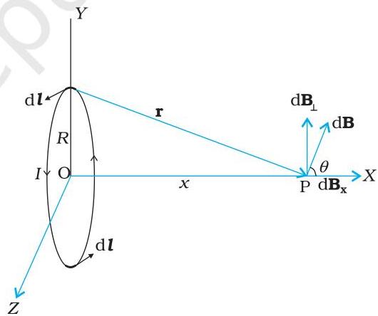 FIGURE 4.9 Magnetic field on the axis of a current carrying circular loop of radius $R$. Shown are the magnetic field $dB$ (due to a line element $dl$) and its components along and perpendicular to the axis.
$ \mathrm {d} B = \frac {\mu_ {0}}{4 \pi} \frac {I \mathrm {d} l}{\left(x ^ {2} + R ^ {2}\right)} \tag {4.9}
$
Figure 4.9 illustrates the orientation of $\mathrm{dB}$. This vector is orthogonal to the plane defined by $\mathrm{d}l$ and $\mathbf{r}$. It possesses a component $\mathrm{dB}_x$ along the $x$-axis and another component perpendicular to the $x$-axis. Upon summation, the components oriented perpendicularly to the $x$-axis mutually cancel, yielding a net zero contribution. Illustratively, the perpendicular component originating from $\mathrm{d}l$ is counteracted by the equivalent component from the diametrically opposite current element, as depicted in Fig. 4.9. Consequently, only the axial ($x$-) component persists. The total magnetic field along the $x$-direction is then derived by integrating the axial component, $\mathrm{dB}_x = \mathrm{dB}\cos \theta$, across the entire loop. As evident from Fig. 4.9,
$ \cos \theta = \frac {R}{\left(x ^ {2} + R ^ {2}\right) ^ {1 / 2}} \tag {4.10} $
From Eqs. (4.9) and (4.10),
$ \mathrm {d} B _ {x} = \frac {\mu_ {0} I \mathrm {d} l}{4 \pi} \frac {R}{\left(x ^ {2} + R ^ {2}\right) ^ {3 / 2}} $
Integrating the infinitesimal elements $\mathrm{d}l$ around the complete loop results in $2\pi R$, which represents the loop's total circumference. Therefore, the magnetic field at point $\mathbf{P}$ generated by the entirety of the circular loop is given by:
$ \mathbf {B} = B _ {x} \hat {\mathbf {i}} = \frac {\mu_ {0} I R ^ {2}}{2 \left(x ^ {2} + R ^ {2}\right) ^ {3 / 2}} \hat {\mathbf {i}} \tag {4.11} $
As a special case of the above result, we may obtain the field at the centre of the loop. Here $x = 0$, and we obtain,
$ \mathbf {B} _ {0} = \frac {\mu_ {0} I}{2 R} \hat {\mathbf {i}} \tag {4.12} $
The magnetic field lines due to a circular wire form closed loops and are shown in Fig. 4.10. The direction of the magnetic field is given by (another) right-hand thumb rule stated below:
Curl the palm of your right hand around the circular wire with the fingers pointing in the direction of the current. The right-hand thumb gives the direction of the magnetic field.
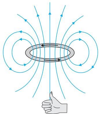 FIGURE 4.10 The magnetic field lines for a current loop. The direction of the field is given by the right-hand thumb rule described in the text. The upper side of the loop may be thought of as the north pole and the lower side as the south pole of a magnet.
Example 4.5 A straight wire carrying a current of $12\mathrm{A}$ is bent into a semi-circular arc of radius $2.0~\mathrm{cm}$ as shown in Fig. 4.11(a). Consider the magnetic field $\mathbf{B}$ at the centre of the arc. (a) What is the magnetic field due to the straight segments? (b) In what way the contribution to $\mathbf{B}$ from the semicircle differs from that of a circular loop and in what way does it resemble? (c) Would your answer be different if the wire were bent into a semi-circular arc of the same radius but in the opposite way as shown in Fig. 4.11(b)?
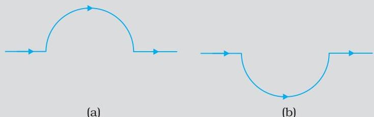 FIGURE 4.11
Solution
(a) For the straight sections, the differential length element $\mathrm{d}l$ is oriented parallel to the position vector $\mathbf{r}$ from the current element to the observation point. Consequently, their cross product, $\mathrm{d}l \times \mathbf{r}$, evaluates to zero. This implies that these rectilinear portions do not generate any magnetic field contribution to the total magnitude |B|. (b) Within the semicircular arc segments, the cross product $\mathrm{d}l \times \mathbf{r}$ maintains a consistent direction, specifically pointing into the plane of the paper. As a result, all individual contributions to the magnetic field sum coherently in magnitude. The resultant direction of the magnetic field $\mathbf{B}$ for a semicircular arc is determined by the right-hand rule, and its magnitude is precisely half that produced by a complete circular loop. Therefore, the magnetic field $\mathbf{B}$ is found to be $1.9 \times 10^{-4} \mathrm{T}$, directed perpendicularly into the plane of the paper. (c) The magnetic field $\mathbf{B}$ in this case possesses an identical magnitude to that described in part (b), but its orientation is diametrically opposite.
Example 4.6 Consider a tightly wound 100 turn coil of radius 10 cm, carrying a current of 1 A. What is the magnitude of the magnetic field at the centre of the coil?
Solution Given that the coil is tightly wound, it is reasonable to assume that each individual circular turn possesses an identical radius, specified as $R = 10 , \text{cm} = 0.1 , \text{m}$. The total count of turns is $N = 100$. The magnitude of the magnetic field at the center is calculated as follows:
$ B = \frac {\mu_ {0} N I}{2 R} = \frac {4 \pi \times 1 0 ^ {- 7} \times 1 0 ^ {2} \times 1}{2 \times 1 0 ^ {- 1}} = 2 \pi \times 1 0 ^ {- 4} = 6. 2 8 \times 1 0 ^ {- 4} \mathrm {T} $
4.6 AMPERE'S CIRCUITAL LAW
The Biot-Savart law can be formulated differently and elegantly. Ampere's circuital law involves an open surface defined by a boundary (refer to Fig. 4.12), through which an electric current flows. This boundary is conceptualized as being composed of numerous infinitesimal line segments. For any given segment of length $dl$, the tangential component of the magnetic field, $B_t$, at that location is determined and then multiplied by the
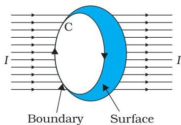 FIGURE 4.12
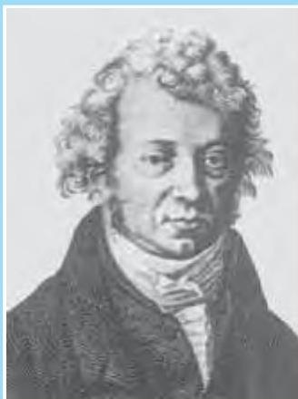
Andre Ampere (1775 - 1836) Andre Marie Ampere was a French physicist, mathematician and chemist who founded the science of electrodynamics. Ampere was a child prodigy who mastered advanced mathematics by the age of 12. Ampere grasped the significance of Oersted's discovery. He carried out a large series of experiments to explore the relationship between current electricity and magnetism. These investigations culminated in 1827 with the publication of the 'Mathematical Theory of Electrodynamic Phenomena Deduced Solely from Experiments'. He hypothesised that all magnetic phenomena are due to circulating electric currents. Ampere was humble and absent-minded. He once forgot an invitation to dine with the Emperor Napoleon. He died of pneumonia at the age of 61. His gravestone bears the epitaph: Tandem Felix (Happy at last).
length of that element $dl$. [Note: $\mathbf{B}_i dl = \mathbf{B} \cdot d\mathbf{l}$ ]. These individual products are then summed. As the lengths of these elements approach zero and their quantity increases indefinitely, this summation converges to an integral. Ampere's law postulates that this integral is equivalent to $\mu_0$ multiplied by the aggregate current traversing the surface; specifically:
$ \oint \mathbf {B} \cdot d \mathbf {l} = \mu_ {0} I \tag {4.13(a)} $
Here, $I$ represents the total electric current penetrating the specified surface. The integration is performed along the closed path that corresponds to the boundary $C$ of the surface. This relationship incorporates a specific sign convention, dictated by the right-hand rule. If the fingers of the right hand are curved in the direction in which the boundary is followed during the line integral $\oint \mathbf{B} \cdot d\mathbf{l}$, then the orientation of the thumb indicates the direction considered positive for the current $I$.
In numerous practical scenarios, a significantly streamlined form of Eq. [4.13(a)] suffices. For these instances, we postulate the ability to select a closed path (termed an amperian loop) such that, at every location along this loop, one of the following conditions holds:
(i) B is tangential to the loop and is a non-zero constant B, or (ii) B is normal to the loop, or (iii) B vanishes.
Consequently, if $L$ denotes the segment of the loop where $B$ is tangential, and $I_e$ represents the current encompassed by the loop, then Eq. (4.13) simplifies to:
$ B L = \mu_ {0} I _ {e} \tag {4.13(b)} $
In scenarios involving inherent symmetry, such as that of an infinitely long, straight current-carrying conductor (as depicted in Fig. 4.13), Ampere's law offers a straightforward method for determining the magnetic field. This application parallels the utility of Gauss's law in simplifying the calculation of electric fields. The principle is illustrated in Example 4.8. For the chosen circular Amperian loop, the magnetic field vector is tangential to its circumference. Applying Ampere's law, the left-hand side of Equation [4.13(b)] evaluates to B ⋅ 2πr. Consequently, the magnetic field at a radial distance $r$ outside the wire is tangential and mathematically defined as:
$ B \times 2 \pi r = \mu_ {0} I, $
$ B = \mu_ {0} I / (2 \pi r) \tag {4.14} $
The derived outcome for an infinite wire presents several noteworthy implications:
(i) This result indicates that the magnetic field maintains a constant magnitude at all points on any circular path of radius $r$ centered on the wire's axis. This characteristic signifies
a cylindrical symmetry in the magnetic field distribution. Consequently, a field typically described by three spatial coordinates becomes dependent solely on the radial distance, $r$. The presence of such symmetry inherently simplifies analytical solutions.
(ii) The orientation of the magnetic field vector at any point on such a circle is tangential to that circle. Consequently, lines of constant magnetic field magnitude trace out concentric circles. As observed in Fig. 4.1(c), iron filings visually confirm these concentric circular patterns. These magnetic field lines form continuous closed loops, a fundamental distinction from electrostatic field lines which originate from positive charges and terminate on negative charges. This derived expression for the magnetic field of a straight wire offers a theoretical underpinning for Oersted's experimental observations. (iii) It is noteworthy that despite the infinite extent of the wire, the magnetic field it produces at any non-zero distance remains finite. The field magnitude approaches infinity only in the immediate vicinity of the wire. Furthermore, the field strength exhibits a direct proportionality to the current flowing through the conductor and an inverse proportionality to the radial distance from this infinitely long current source. (iv) A straightforward mnemonic exists for ascertaining the magnetic field's direction around a long wire. This principle, known as the right-hand rule*, states:
Grasp the wire in your right hand with your extended thumb pointing in the direction of the current. Your fingers will curl around in the direction of the magnetic field.
Ampere's circuital law does not introduce fundamentally new physical content compared to the Biot-Savart law. Both formulations establish a relationship between the magnetic field and the current, and both elucidate identical physical phenomena arising from a steady electrical current. The relationship between Ampere's law and Biot-Savart law is analogous to that between Gauss's law and Coulomb's law. In both cases, Ampere's and Gauss's laws connect a physical quantity observed at the periphery or boundary (specifically, the magnetic or electric field) to its corresponding source quantity located within the enclosed interior region (i.e., current or charge). It is further important to note that Ampere's circuital law is valid exclusively for steady currents, meaning those that exhibit no temporal fluctuations. The subsequent example will clarify the precise definition of the term "enclosed current."
Example 4.7 Consider a lengthy, straight conductor possessing a circular cross-section (with radius $a$), through which a constant current $I$ flows. This current $I$ is distributed uniformly throughout the conductor's cross-sectional area. Determine the magnetic field strength in the regions where $r < a$ and $r > a$.
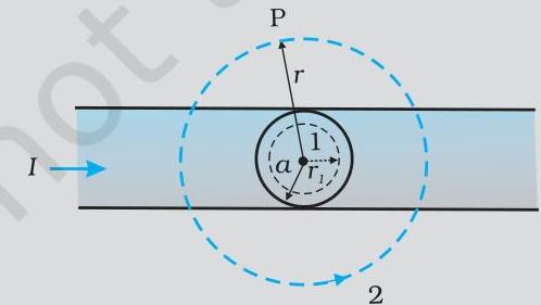 FIGURE 4.13
Solution (a) For the scenario where $r > a$, we select an
Amperian loop, designated as loop 2, which is a circle concentrically aligned with the conductor's cross-section. For this chosen loop, its circumference is given by:
$ L = 2 \pi r $
The total current encompassed by this loop, $I_c$, is the entire current $I$ flowing through the wire. Thus, $I_c = I$. Applying Ampere's circuital law yields the well-known formula for the magnetic field generated by an infinitely long straight conductor:
$ B (2 \pi r) = \mu_ {0} I $
Consequently, the magnetic field strength is:
$ B = \frac {\mu_ {0} I}{2 \pi r} \quad [ 4.15 (\mathrm {a}) ] $
This indicates a proportionality:
$ B \propto \frac {1}{r} \quad (r > a) $
Conversely, for the region $r < a$, the current enclosed, $I_c$, is no longer the total current $I$, but rather a fraction of it. Due to the uniform current density across the cross-section, the enclosed current can be calculated as the ratio of the areas:
$ I _ {c} = I \left(\frac {\pi r ^ {2}}{\pi a ^ {2}}\right) = \frac {I r ^ {2}}{a ^ {2}} $
Applying Ampere's law with this modified enclosed current yields:
$ B(2\pi r) = \mu_0\frac{Ir^2}{a^2} $
From this, the magnetic field strength is derived as:
$ B = \left(\frac {\mu_ {0} I}{2 \pi a ^ {2}}\right) r \tag {4.15(b)} $
Thus, the magnetic field exhibits a direct proportionality:
$ B \propto r \quad (r < a) $
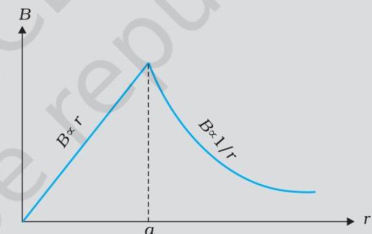 FIGURE 4.14
The accompanying Figure (4.14) illustrates the variation in the magnitude of the magnetic field $\mathbf{B}$ as a function of the radial distance $r$ from the wire's central axis. The magnetic field's orientation is tangential to each corresponding circular Amperian loop (either 1 or 2) and is determined by the right-hand rule as previously outlined in this chapter. This particular problem benefits from sufficient symmetry, thereby allowing for a straightforward application of Ampere's circuital law. It is crucial to recognize that although Ampere's circuital law is universally valid for any closed loop, it does not consistently simplify the determination of the magnetic field in all circumstances. For instance, in the context of the circular loop examined in Section 4.5, this law cannot be employed to readily derive the straightforward expression $B = \mu_0 I / 2R$ [Eq. (4.12)] for the magnetic field at the loop's center. Nevertheless, for numerous scenarios characterized by a high degree of symmetry, Ampere's law proves to be an exceedingly practical tool. In the subsequent section, we will utilize this principle to compute the magnetic field generated by a frequently employed and highly effective magnetic configuration: the solenoid.
4.7 THE SOLENOID
This section focuses on the characteristics of a long solenoid. A long solenoid is defined as one whose axial dimension significantly exceeds its radial dimension. Its structure comprises an extended wire coiled helically, with adjacent windings positioned in close proximity. Consequently, each individual turn can be conceptualized as a circular current loop. The resultant magnetic field represents the vector superposition of the fields generated by all constituent turns. To ensure electrical isolation between turns, insulated (e.g., enamelled) wires are employed for the winding.
(a)
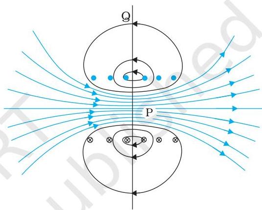
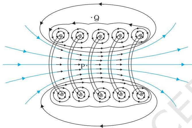 (b) The magnetic field of a finite solenoid.
 (b)
FIGURE 4.15 (a) The magnetic field due to a section of the solenoid which has been stretched out for clarity. Only the exterior semi-circular part is shown. Notice how the circular loops between neighbouring turns tend to cancel.
(b)
FIGURE 4.15 (a) The magnetic field due to a section of the solenoid which has been stretched out for clarity. Only the exterior semi-circular part is shown. Notice how the circular loops between neighbouring turns tend to cancel.
The magnetic field configuration of a finite solenoid is illustrated in Figure 4.15. An magnified view of a segment of this solenoid is presented in Fig. 4.15(a). Figure 4.15(b) depicts the complete finite solenoid along with its associated magnetic field. Observation of the circular loops in Fig. 4.15(a) reveals the cancellation of the magnetic field components between adjacent turns. Within Fig. 4.15(b), it is evident that the magnetic field at the interior central point $\mathbf{P}$ exhibits characteristics of uniformity, high magnitude, and axial alignment. Conversely, the field at the exterior central point $\mathbf{Q}$ is comparatively feeble and also oriented along the solenoid's axis, lacking any transverse or normal component. As the
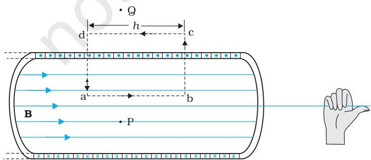 FIGURE 4.16 The magnetic field of a very long solenoid. We consider a rectangular Amperian loop abcd to determine the field.
solenoid's length is increased, it approximates an idealized, infinitely long cylindrical current sheet. This idealized scenario is depicted in Figure 4.16. The magnetic field external to such a solenoid tends towards zero; for practical purposes, we will consider it to be negligible. Internally, the magnetic field lines become uniformly parallel to the central axis.
Let us analyze a rectangular Amperian contour, designated abcd. As previously established, the magnetic field along the segment cd is null. For the transverse segments bc and ad, the field component perpendicular to the path is zero; consequently, these sections do not contribute to the line integral. Assuming the magnetic field along ab is $B$, the effective length of the Amperian loop for integration becomes $L = h$.
If $n$ denotes the turn density (number of turns per unit length), then the cumulative number of turns within the length $h$ is $nh$. The total current enclosed by the loop, $I_{e}$, is thus $I(nh)$, where $I$ represents the current flowing through each turn of the solenoid. Applying Ampere's circuital law [referencing Eq. 4.13 (b)]:
$ BL = \mu_{0} I_{e}, \quad Bh = \mu_{0} I(n h) $
$ B = \mu_{0} n I \tag{4.16} $
The orientation of the magnetic field can be determined using the right-hand rule. Solenoids are frequently employed to generate spatially uniform magnetic fields. As will be explored in the subsequent chapter, the magnitude of this field can be significantly enhanced by incorporating a soft iron core within the solenoid's interior.
EXAMPLE 4.17
Example 4.8 A solenoid of length $0.5,\mathrm{m}$ has a radius of $1,\mathrm{cm}$ and is made up of 500 turns. It carries a current of 5 A. What is the magnitude of the magnetic field inside the solenoid?
To begin the solution, the turns per unit length are calculated as:
$ n = \frac{500}{0.5} = 1000,\mathrm{turns/m} $
Given the solenoid's length $l = 0.5,\mathrm{m}$ and radius $r = 0.01,\mathrm{m}$, the ratio $l/a$ is $50$, indicating that $l \gg a$. Therefore, the formula for a long solenoid, as presented in Eq. (4.16), can be utilized:
$ \begin{array}{l} B = \mu_{0} n I \ = 4\pi \times 10^{-7} \times 10^{3} \times 5 \ = 6.28 \times 10^{-3} ,\mathrm{T} \end{array} $
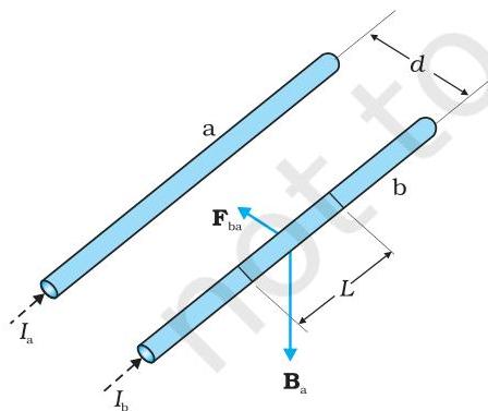 FIGURE 4.17 Two long straight parallel conductors carrying steady currents $I_{\mathrm{a}}$ and $I_{\mathrm{b}}$ and separated by a distance $d$. $\mathbf{B}_{\mathrm{a}}$ is the magnetic field set up by conductor 'a' at conductor 'b'.
4.8 FORCE BETWEEN TWO PARALLEL CURRENTS, THE AMPERE
Our prior understanding establishes the presence of a magnetic field generated by a current-carrying conductor, consistent with the Biot-Savart law. Moreover, we know that a conductor carrying current experiences a force when situated in an external magnetic field, a phenomenon described by the Lorentz force equation. Consequently, it is reasonable to infer that mutual magnetic forces will arise between two current-carrying conductors positioned in proximity. During the years 1820-1825, Ampere meticulously investigated the characteristics of this magnetic interaction, including its reliance on current magnitude, conductor geometry, and the separation between conductors. This section will focus on the straightforward case of two parallel current-carrying conductors, an illustration that may aid in appreciating the rigor of Ampere's contributions.
As depicted in Figure 4.17, two elongated, parallel conductors, designated 'a' and 'b', are positioned a distance $d$ apart, carrying parallel currents $I_a$ and $I_b$, respectively. Conductor 'a' generates a uniform magnetic field, denoted $\mathbf{B}_a$, across all points along conductor 'b'. Employing the right-hand rule, the orientation of this field is determined to be downward (assuming horizontal placement of the conductors). Its magnitude can be derived either from Eq. [4.15(a)] or Ampere's circuital law, and is expressed as:
$ B_a = \frac{\mu_0 I_a}{2\pi d} $
Consequently, conductor 'b', which carries current $I_b$, will be subjected to a lateral force originating from the field $\mathbf{B}a$. The direction of this force is directed towards conductor 'a' (this can be confirmed). This force is denoted as $\mathbf{F}{ba}$, representing the force exerted on a segment of length $L$ of conductor 'b' by conductor 'a'. The magnitude of this force is defined by Eq. (4.4) as:
$ \begin{array}{l} F_{ba} = I_b L B_a \ = \frac{\mu_0 I_a I_b}{2\pi d} L \tag{4.17} \end{array} $
Naturally, the force exerted on conductor 'a' by conductor 'b' can also be calculated. Through analogous reasoning, we can determine the force $\mathbf{F}{ab}$, which acts on a segment of length $L$ of 'a' due to the current in 'b'. This force is equal in magnitude to $F{ba}$ but is directed towards 'b'. Hence, the relationship is:
$ \mathbf{F}{ba} = -\mathbf{F}{ab} \tag{4.18} $
It is noteworthy that this outcome aligns with Newton's third Law. Therefore, for the specific scenario of parallel conductors with steady currents, we have demonstrated that the Biot-Savart law and the Lorentz force collectively produce results consistent with Newton's third Law*.
As previously established, electrical currents moving in the same direction exert an attractive force upon one another. Conversely, it can be demonstrated that currents flowing in opposing directions experience a repulsive force. Consequently, the principle states:
Parallel currents attract, and antiparallel currents repel.
This interaction fundamentally contrasts with the behavior observed in electrostatics. In electrostatics, charges of identical sign (like charges) repel; however, in magnetostatics, currents flowing in parallel (like currents) exhibit mutual attraction.
Let $f_{ba}$ denote the magnitude of the force $\mathbf{F}_{ba}$ exerted per unit length. Based on Eq. (4.17), this is given by:
$ f_{ba} = \frac{\mu_0 I_a I_b}{2\pi d} \tag{4.19} $
This formula serves as the basis for defining the ampere (A), which stands as one of the seven fundamental SI units.
The ampere is defined as the magnitude of that constant current which, if present in each of two infinitely long, straight, parallel conductors of negligible cross-sectional area, positioned precisely one meter apart in a vacuum, would induce a force between them amounting to exactly $2 \times 10^{-7}$ newtons per meter of length.
This specific definition of the ampere was formally established in 1946. While fundamentally theoretical, its practical realization necessitates the mitigation of Earth's magnetic field interference and the replacement of idealized infinitely long wires with precisely engineered multiturn coils. The measurement of this resultant mechanical force is typically performed using a device known as a current balance.
The coulomb, which is the SI unit for electric charge, can subsequently be defined using the ampere.
Specifically, if a constant current of 1 ampere flows through a conductor, the amount of electric charge passing through its cross-section within a duration of 1 second is defined as one coulomb (1C).
Example 4.9 At a particular location, the horizontal component of Earth's magnetic field measures $3.0 \times 10^{-5} \mathrm{T}$, with its orientation extending from geographic south towards geographic north. A prolonged, straight conductor is carrying a constant current of 1A. Determine the force per unit length acting on this conductor when it rests on a horizontal surface, given that the current's direction is (a) from east to west; (b) from south to north?
$ \text{Solution } \mathbf{F} = I\mathbf{l} \times \mathbf{B} $
$ F = I B \sin \theta $
The force exerted per unit length is therefore expressed as:
$ f = F / l = I B \sin \theta $
(a) Considering the scenario where the current flows from east to west:
$ \theta = 90^{\circ} $
Consequently, the force per unit length is:
$ \begin{array}{l} f = I B \ = 1 \times 3 \times 10^{-5} = 3 \times 10^{-5} \mathrm{N \ m^{-1}} \end{array} $
This calculated value significantly exceeds the $2 \times 10^{-7} \mathrm{Nm}^{-1}$ specified in the official definition of the ampere. Therefore, it is crucial to nullify the influence of Earth's magnetic field and any other extraneous magnetic fields when establishing the standard for the ampere.
The resultant force acts in a downward direction. This directional aspect can be ascertained through the vector cross product's inherent properties.
(b) In the case where the current is directed from south to north:
$ \theta = 0^{\circ} $
$ f = 0 $
Accordingly, no force is exerted upon the conductor under these conditions.
4.9 TORQUE ON CURRENT LOOP, MAGNETIC DIPOLE
4.9.1 Torque on a rectangular current loop in a uniform magnetic field
This section demonstrates that a rectangular loop, which carries a constant current $I$ and is situated within a uniform magnetic field, is subjected to a torque rather than a net translational force. This phenomenon exhibits a parallel to the behavior of an electric dipole when positioned within a uniform electric field (refer to Section 1.11).
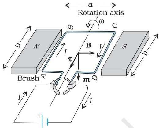
Initially, we examine a straightforward scenario where the rectangular loop is positioned such that the uniform magnetic field $\mathbf{B}$ lies entirely within the plane of the loop, as depicted in Fig. 4.18(a).
The magnetic field applies no force to the arms AD and BC of the loop. Conversely, it acts perpendicularly upon arm AB, generating a force $\mathbf{F}_1$ directed into the plane of the loop. The magnitude of this force is expressed as:
$ F_1 = I b B $
In a comparable manner, a force $\mathbf{F}_2$ is exerted on arm CD, with its direction pointing out of the plane of the paper.
$ F_2 = I b B = F_1 $
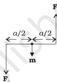
Consequently, the aggregate force acting on the loop is zero. However, a torque is produced on the loop by the coupled forces $\mathbf{F}_1$ and $\mathbf{F}_2$. A perspective of the loop from the AD end, presented in Figure 4.18(b), illustrates that this torque induces an anticlockwise rotation. The magnitude of this torque is calculated as:
$ \begin{array}{l} \tau = F_1 \frac{a}{2} + F_2 \frac{a}{2} \ = I b B \frac{a}{2} + I b B \frac{a}{2} = I (a b) B \ = I A B \tag{4.20} \end{array} $
where $A = ab$ denotes the enclosed area of the rectangular loop.
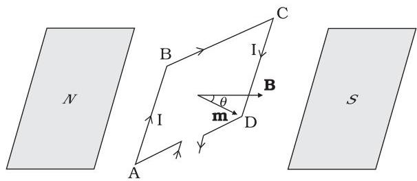
Subsequently, we examine the scenario where the plane of the loop is not aligned with the magnetic field, but instead forms an angle with it. We define $\theta$ as the angle between the magnetic field and the normal vector to the coil's plane (the preceding case corresponds to $\theta = \pi / 2$). This more general configuration is depicted in Figure 4.19.
The forces acting upon arms BC and DA are of equal magnitude, opposite in direction, and operate along the coil's central axis, which links the centers of mass of BC and DA. Since these forces are collinear, they mutually cancel, yielding no net force or torque. Forces $\mathbf{F}_1$ and $\mathbf{F}_2$ are exerted on arms AB and CD, respectively. These forces are also equal in magnitude and opposite in direction, with their magnitude given by:
$ F_1 = F_2 = I b B $
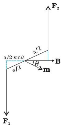
Crucially, these forces are not collinear, thereby forming a couple, consistent with the previous analysis. Nevertheless, the resulting torque is diminished compared to the initial scenario where the loop's plane was aligned with the magnetic field. This reduction occurs because the perpendicular separation between the forces of the couple has been reduced. Figure 4.19(b) provides an AD-end perspective of this configuration, elucidating the two forces that constitute the couple. The magnitude of the torque exerted on the loop is determined by:
$ \begin{array}{l} \tau = F_1 \frac{a}{2} \sin \theta + F_2 \frac{a}{2} \sin \theta \ = I a b B \sin \theta \ = I A B \sin \theta \tag{4.21} \end{array} $
 (a)
(a)
 (b)
FIGURE 4.18 (a) Depiction of a rectangular coil carrying current within a uniform magnetic field. The magnetic moment is oriented downward. The torque $\tau$ is directed along the axis and induces an anticlockwise rotation of the coil. (b) Illustration of the couple of forces acting on the coil.
(b)
FIGURE 4.18 (a) Depiction of a rectangular coil carrying current within a uniform magnetic field. The magnetic moment is oriented downward. The torque $\tau$ is directed along the axis and induces an anticlockwise rotation of the coil. (b) Illustration of the couple of forces acting on the coil.
Physics
 (a)
(a)
 (b)
FIGURE 4.19 (a) The area vector of the loop ABCD forms an arbitrary angle $\theta$ with the magnetic field. (b) Top view of the loop, illustrating the forces $\mathbf{F}_1$ and $\mathbf{F}_2$ acting on arms AB and CD.
(b)
FIGURE 4.19 (a) The area vector of the loop ABCD forms an arbitrary angle $\theta$ with the magnetic field. (b) Top view of the loop, illustrating the forces $\mathbf{F}_1$ and $\mathbf{F}_2$ acting on arms AB and CD.
As $\theta \rightarrow 0$, the perpendicular separation between the forces constituting the couple also diminishes to zero. This renders the forces collinear, leading to a net force and torque of zero. The torques described in Eqs. (4.20) and (4.21) can be expressed as the vector product of the coil's magnetic moment and the magnetic field. We define the magnetic moment of the current loop as:
$ \mathbf {m} = I \mathbf {A} \tag {4.22} $
where the orientation of the area vector $\mathbf{A}$ is determined by the right-hand thumb rule, pointing into the plane of the paper in Fig. 4.18. Consequently, given that $\theta$ represents the angle between $\mathbf{m}$ and $\mathbf{B}$, Eqs. (4.20) and (4.21) can be unified into a single expression:
$ \boldsymbol {\tau} = \mathbf {m} \times \mathbf {B} \tag {4.23} $
This is analogous to the electrostatic case (an electric dipole with dipole moment $\mathbf{p}_e$ in an electric field $\mathbf{E}$).
$ \tau = \mathbf {p} _ {e} \times \mathbf {E} $
As is evident from Eq. (4.22), the magnetic moment possesses dimensions of $[\mathrm{A}][\mathrm{L}^2]$, and its standard unit is $\mathrm{Am}^2$.
From Eq. (4.23), it is observed that the torque $\pmb{\tau}$ becomes zero when $\mathbf{m}$ is either parallel or antiparallel to the magnetic field $\mathbf{B}$. This condition signifies an equilibrium state, as no torque acts upon the coil (a principle applicable to any entity possessing a magnetic moment $\mathbf{m}$). When $\mathbf{m}$ and $\mathbf{B}$ are parallel, the equilibrium is stable. Any minor rotation of the coil generates a restoring torque that returns it to its initial configuration. Conversely, if they are antiparallel, the equilibrium is unstable, as any rotation induces a torque that amplifies with the degree of displacement. The existence of this torque also explains why a small magnet or any magnetic dipole aligns itself with an external magnetic field.
If the loop comprises $N$ closely wound turns, the expression for torque, Eq. (4.23), remains valid, with
$ \mathbf {m} = N I \mathbf {A} \tag {4.24} $
Example 4.10 A 100-turn closely wound circular coil of radius 10 cm, carries a current of 3.2 A. (a) What is the magnetic field strength at the coil's center? (b) What is the magnetic moment of this coil?
The coil is positioned in a vertical plane and is free to rotate about a horizontal axis that coincides with its diameter. A uniform magnetic field of 2T, directed horizontally, is present such that the coil's axis is initially aligned with the field. The coil then rotates through an angle of $90^{\circ}$ under the influence of the magnetic field. (c) What are the magnitudes of the torques acting on the coil at its initial and final positions? (d) What angular speed does the coil acquire after rotating by $90^{\circ}$? The moment of inertia of the coil is $0.1\mathrm{kg}\mathrm{m}^{2}$.
Solution
(a) The magnetic field strength at the center of a circular coil can be determined using Equation (4.12):
$ B = \frac {\mu_ {0} N I}{2 R} $
Given the parameters: $N = 100$ (number of turns), $I = 3.2$ A (current), and $R = 0.1$ m (radius). Substituting these values yields:
$ \begin{array}{l} B = \frac {4 \pi \times 1 0 ^ {- 7} \times 3 . 2}{2 \times 1 0 ^ {- 1}} = \frac {4 \times 1 0 ^ {- 5} \times 1 0}{2 \times 1 0 ^ {- 1}} \quad (\text {using} \pi \times 3. 2 = 1 0) \ = 2 \times 1 0 ^ {- 3} \mathrm {T} \ \end{array} $
The orientation of this magnetic field is established by applying the right-hand thumb rule.
(b) The magnetic moment, as defined by Equation (4.24), is calculated as:
$ m = N I A = N I \pi r ^ {2} = 1 0 0 \times 3. 2 \times 3. 1 4 \times 1 0 ^ {- 2} = 1 0 \mathrm {A m} ^ {2} $
Its direction is similarly determined using the right-hand thumb rule.
(c) The torque $\tau$ experienced by the coil is given by the magnitude of the cross product of the magnetic moment and the magnetic field, as per Equation (4.23): $\tau = |\mathbf{m}\times \mathbf{B}|$.
$ = m B \sin \theta $
At the outset, the angle $\theta$ is $0$, resulting in an initial torque $\tau_{t} = 0$. Subsequently, the angle becomes $\theta = \pi /2$ (or $90^{\circ}$), leading to a final torque $\tau_{t} = mB = 10\times 2 = 20\mathrm{Nm}$.
(d) Applying Newton's second law to rotational motion, the equation of motion is:
$ \beta \frac {\mathrm {d} \omega}{\mathrm {d} t} = m B \sin \theta $
Here, $\beta$ represents the moment of inertia of the coil. By employing the chain rule for differentiation, the term $\frac {\mathrm {d} \omega}{\mathrm {d} t}$ can be expressed as:
$ \frac {\mathrm {d} \omega}{\mathrm {d} t} = \frac {\mathrm {d} \omega}{\mathrm {d} \theta} \frac {\mathrm {d} \theta}{\mathrm {d} t} = \frac {\mathrm {d} \omega}{\mathrm {d} \theta} \omega $
Substituting this into the previous equation allows us to reformulate it as:
$ \beta \omega \mathrm {d} \omega = m B \sin \theta \mathrm {d} \theta $
To determine the final angular velocity, this equation is integrated from an initial angle of $\theta = 0$ to a final angle of $\theta = \pi /2$:
$ \begin{array}{l} \beta \int_ {0} ^ {\omega_ {f}} \omega d \omega = m B \int_ {0} ^ {\pi / 2} \sin \theta d \theta \ \beta \frac {\omega_ {f} ^ {2}}{2} = - m B \cos \theta | _ {0} ^ {\pi / 2} = m B \ \omega_ {f} = \left(\frac {2 m B}{\beta}\right) ^ {1 / 2} = \left(\frac {2 \times 2 0}{1 0 ^ {- 1}}\right) ^ {1 / 2} = 2 0 \mathrm {s} ^ {- 1} \ \end{array} $
Example 4.11
(a) A circular loop carrying an electric current is situated on a smooth horizontal surface. Is it possible to establish a uniform magnetic field in such a way that the loop rotates about its own vertical axis? (b) A circular loop, carrying current, is positioned within a uniform external magnetic field. If the loop is free to rotate, what configuration represents its stable equilibrium? Demonstrate that in this particular orientation, the magnetic flux of the combined field (comprising the external field and the field generated by the loop) reaches its maximum value. (c) An irregularly shaped current-carrying loop is placed in an external magnetic field. If the wire is flexible, why does it transform into a circular shape?
Solution
(a) No, this is not feasible because such a rotation would necessitate the torque, $\tau$, to be oriented vertically. However, the torque is defined as $\tau = I\mathbf{A} \times \mathbf{B}$. Given that the area vector $\mathbf{A}$ of a horizontal loop points in the vertical direction, the resultant torque $\tau$ would always lie within the plane of the loop, regardless of the orientation of $\mathbf{B}$.
(b) The stable equilibrium orientation occurs when the loop's area vector $\mathbf{A}$ is aligned precisely with the direction of the external magnetic field. In this configuration, the magnetic field generated by the loop itself is parallel to the external field, with both fields oriented perpendicularly to the loop's plane. This alignment results in the maximization of the total magnetic flux.
(c) A flexible loop adopts a circular shape with its plane perpendicular to the magnetic field to maximize the magnetic flux. This phenomenon occurs because, for a given perimeter length, a circle encloses the largest possible area compared to any other geometric shape.
4.9.2 Circular current loop as a magnetic dipole
This section focuses on the current loop, which serves as a fundamental magnetic element. Our aim is to illustrate that the magnetic field generated by a circular current loop, particularly at considerable distances, exhibits characteristics remarkably analogous to the electric field produced by an electric dipole. As established in Section 4.5, the magnetic field along the axis of a circular loop with radius $R$, carrying a steady current $I$, has a magnitude given by [(Eq. (4.11)],
$ B = \frac{\mu_0 I R^2}{2 (x^2 + R^2)^{3/2}} $
The field's orientation is axial, determined by the right-hand thumb rule (Fig. 4.10). In this context, $x$ represents the axial distance from the loop's geometric center. When considering points significantly far from the loop, i.e., $x \gg R$, the $R^2$ term in the denominator can be neglected. Consequently,
$ B = \frac{\mu_0 I R^2}{2 x^3} $
It is important to recognize that the loop's area, $A$, is defined as $\pi R^2$. Therefore,
$ B = \frac{\mu_0 I A}{2 \pi x^3} $
Consistent with previous definitions, the magnetic moment $\mathbf{m}$ is characterized by a magnitude of $IA$, such that $\mathbf{m} = IA$. This leads to:
$ \begin{array}{l} B = \frac{\mu_0 m}{2 \pi x^3} \ = \frac{\mu_0}{4 \pi} \frac{2 \mathbf{m}}{x^3} \tag{4.25(a)} \end{array} $
Equation [4.25(a)] bears a strong resemblance to a previously derived expression for the electric field of a dipole. This analogy becomes apparent upon performing the following substitutions:
$ \mu_0 \rightarrow 1 / \varepsilon_0 $
$ \mathbf{m} \rightarrow \mathbf{p}_e \text{ (electrostatic dipole)} $
$ \mathbf{B} \rightarrow \mathbf{E} \text{ (electrostatic field)} $
Applying these transformations yields:
$ \mathbf {E} = \frac {2 \mathbf {p} _ {e}}{4 \pi \varepsilon_ {0} x ^ {3}} $
This expression corresponds exactly to the on-axis electric field of an electric dipole, as discussed in Chapter 1, Section 1.9 [Eq. (1.20)].
The aforementioned analogy extends beyond this specific case. In Chapter 1, we determined that the electric field along the perpendicular bisector of a dipole is given by [See Eq.(1.21)],
$ E \simeq \frac {\mathbf {p} _ {e}}{4 \pi \varepsilon_ {0} x ^ {3}} $
with $x$ denoting the separation from the dipole. Should we substitute $\mathbf{p} \rightarrow \mathbf{m}$ and $\mu_0 \rightarrow 1 / \varepsilon_0$ into this equation, the resulting expression for $\mathbf{B}$ describes the field at a point within the loop's plane, at a distance $x$ from its center. This holds true for $x >> R$,
$
\mathbf {B} \simeq \frac {\mu_ {0}}{4 \pi} \frac {\mathbf {m}}{x ^ {3}}; \quad x >> R \tag {4.25(b)} $
These results, presented in Eqs. [4.25(a)] and [4.25(b)], achieve exactness when applied to an idealized point magnetic dipole.
It can be demonstrated that the preceding findings are applicable to any planar loop; specifically, a planar current loop behaves as a magnetic dipole characterized by a dipole moment $\mathbf{m} = I\mathbf{A}$, serving as the magnetic counterpart to the electric dipole moment $\mathbf{p}$. Nevertheless, a crucial distinction exists: an electric dipole is constituted by two fundamental units, namely electric charges (or electric monopoles). Conversely, in the realm of magnetism, the magnetic dipole (or a current loop) represents the most fundamental constituent. The existence of magnetic monopoles, which would be analogous to electric charges, remains unconfirmed.
Our previous discussions established that a current loop (i) generates a magnetic field (refer to Fig. 4.10) and behaves as a magnetic dipole when observed from considerable distances, and (ii) experiences a rotational force akin to a magnetic needle. This observation prompted Ampere to hypothesize that all magnetic phenomena originate from circulating electric currents. While this proposition holds partial validity, magnetic monopoles have yet to be empirically detected. Nevertheless, fundamental particles such as electrons and protons possess an inherent magnetic moment that cannot be attributed solely to circulating currents.
4.10 THE MOVING COIL GALVANOMETER
The characteristics of currents and voltages within electrical circuits were thoroughly examined in Chapters 3. However, the crucial question remains: how are these quantities measured? What methodology allows us to assert that a circuit carries a current of $1.5\mathrm{A}$ or that a resistor exhibits a voltage drop of $1.2\mathrm{V}$? Figure 4.20 illustrates a highly effective device designed for this purpose: the moving coil galvanometer (MCG). Its operational principles can be elucidated by drawing upon the concepts explored in Section 4.9.
The galvanometer comprises a coil, featuring numerous turns, engineered to rotate freely around a fixed axis (Fig. 4.20) within a uniform radial magnetic field. An integral cylindrical soft iron core serves a dual function: it not only ensures the radial orientation of the magnetic field but also intensifies its strength. When an electric current traverses the coil, it induces a torque upon it. According to Eq. (4.20), this torque is expressed as
$ \tau = N I A B $
Physics
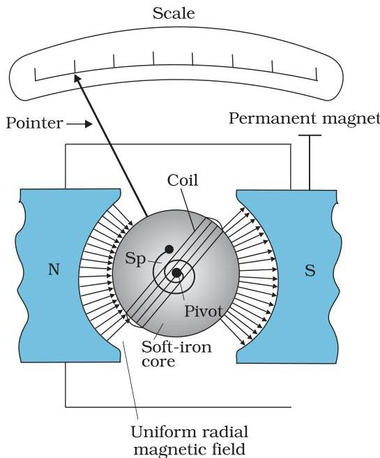 FIGURE 4.20 The moving coil galvanometer. Its elements are described in the text. Depending on the requirement, this device can be used as a current detector or for measuring the value of the current (ammeter) or voltage (voltmeter).
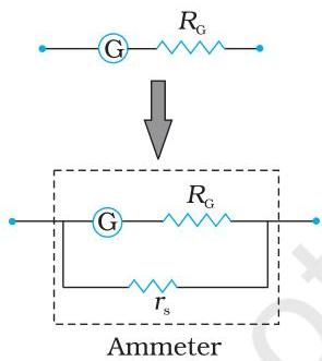 FIGURE 4.21 Conversion of a galvanometer (G) to an ammeter by the introduction of a shunt resistance $r_{s}$ of very small value in parallel.
where the symbols have their usual meaning. Since the field is radial by design, we have taken $\sin \theta = 1$ in the above expression for the torque. The magnetic torque $NIAB$ tends to rotate the coil. A spring $S_{\mathrm{p}}$ provides a counter torque $k\phi$ that balances the magnetic torque $NIAB$ ; resulting in a steady angular deflection $\phi$ . In equilibrium
$ k \phi = N I A B $
where $k$ is the torsional constant of the spring; i.e. the restoring torque per unit twist. The deflection $\phi$ is indicated on the scale by a pointer attached to the spring. We have
$ \phi = \left(\frac {N A B}{k}\right) I \tag {4.26} $
The quantity in brackets is a constant for a given galvanometer.
The galvanometer can be used in a number of ways. It can be used as a detector to check if a current is flowing in the circuit. We have come across this usage in the Wheatstone's bridge arrangement. In this usage the neutral position of the pointer (when no current is flowing through the galvanometer) is in the middle of the scale and not at the left end as shown in Fig.4.20. Depending on the direction of the current, the pointer's deflection is either to the right or the left.
The galvanometer cannot as such be used as an ammeter to measure the value of the current in a given circuit. This is for two reasons: (i) Galvanometer is a very sensitive device, it gives a full-scale deflection for a current of the order of $\mu A$ . (ii) For measuring currents, the galvanometer has to be connected in series, and as it has a large resistance, this will change the value of the current in the circuit. To overcome these difficulties, one attaches a small resistance $r_{s}$ called shunt resistance, in parallel with the galvanometer coil; so that most of the current passes through the shunt. The resistance of this arrangement is,
$ R _ {G} r _ {s} / \left(R _ {G} + r _ {s}\right) = r _ {s} \quad \text {if} \quad R _ {G} >> r _ {s} $
If $r_s$ has small value, in relation to the resistance of the rest of the circuit $R_c$ , the effect of introducing the measuring instrument is also small and negligible. This arrangement is schematically shown in Fig. 4.21. The scale of this ammeter is calibrated and then graduated to read off the current value with ease. We define the current sensitivity of the galvanometer as the deflection per unit current. From Eq. (4.26) this current sensitivity is,
$ \frac {\phi}{I} = \frac {N A B}{k} \tag {4.27} $
Manufacturers can readily enhance sensitivity by augmenting the number of turns, $N$. The selection of galvanometers is based on achieving sensitivity levels appropriate for the experimental requirements.
A galvanometer also serves as a voltmeter for determining potential difference across a specific circuit segment. To function as such, it necessitates a parallel connection across the circuit portion in question. Moreover, it is crucial that it draws minimal current; otherwise, the voltage reading would significantly perturb the circuit's original configuration. Typically, the disruption caused by
the measurement instrument is desired to be less than one percent. To achieve this, a substantial resistance, $R$, is placed in series with the galvanometer. This configuration is graphically represented in Fig. 4.22. It should be noted that the total resistance of the resulting voltmeter becomes:
$ R_{G} + R = R: \text{large} $
The voltmeter's scale is calibrated for straightforward interpretation of voltage values. Voltage sensitivity is defined as the angular deflection observed per unit of applied voltage. As derived from Equation (4.26),
$ \frac{\phi}{V} = \left(\frac{NAB}{k}\right) \frac{I}{V} = \left(\frac{NAB}{k}\right) \frac{1}{R} \tag{4.28} $
It is noteworthy that an enhancement in current sensitivity does not invariably lead to a proportional increase in voltage sensitivity. Consider Equation (4.27), which quantifies current sensitivity. Should the number of turns, $N$, be doubled to $2N$, then:
$ \frac{\phi}{I} \rightarrow 2 \frac{\phi}{I} $
Consequently, the current sensitivity is augmented twofold. Nevertheless, the galvanometer's internal resistance is also expected to double, owing to its direct proportionality with the wire's length. Therefore, when substituting $N \rightarrow 2N$ and $R \rightarrow 2R$ into Equation (4.28), the voltage sensitivity:
$ \frac{\phi}{V} \rightarrow \frac{\phi}{V} $
persists without alteration. Hence, the structural modifications required to transform a galvanometer into an ammeter generally differ from those necessary for its conversion into a voltmeter.
Example 4.12 For the circuit illustrated in Fig. 4.23, the objective is to determine the current value. Calculate the current if the depicted ammeter is (a) a galvanometer possessing an internal resistance $R_{G} = 60.00\ \Omega$; (b) the galvanometer from part (a) modified into an ammeter using a shunt resistance $r_{s} = 0.02\ \Omega$; (c) an ideal ammeter characterized by zero resistance.
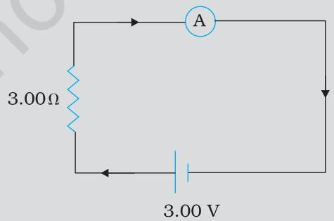 FIGURE 4.23
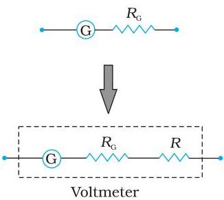 FIGURE 4.22 Conversion of a galvanometer (G) to a voltmeter by the introduction of a resistance $R$ of large value in series.
Solution
(a) The overall resistance within the circuit measures,
$ R _ {\mathrm {G}} + 3 = 6 3 \Omega . \text {Consequently}, I = 3 / 6 3 = 0. 0 4 8 \mathrm {A}. $
(b) The resistance of the galvanometer, when configured as an ammeter, is determined as:
$ \frac {R _ {\mathrm {G}} r _ {\mathrm {s}}}{R _ {\mathrm {G}} + r _ {\mathrm {s}}} = \frac {6 0 \Omega \times 0 . 0 2 \Omega}{(6 0 + 0 . 0 2) \Omega} = 0. 0 2 \Omega $
The aggregate circuit resistance then becomes,
$ 0. 0 2 \Omega + 3 \Omega = 3. 0 2 \Omega . \text {Therefore}, I = 3 / 3. 0 2 = 0. 9 9 \mathrm {A}. $
(c) In the case of an ideal ammeter, possessing negligible resistance,
$ I = 3 / 3 = 1. 0 0 \mathrm {A} $
SUMMARY
- The Lorentz force denotes the resultant force exerted on a charge $q$ traversing with velocity $\mathbf{v}$ through concurrent magnetic ($\mathbf{B}$) and electric ($\mathbf{E}$) fields. Its mathematical representation is:
$ \mathbf {F} = q (\mathbf {v} \times \mathbf {B} + \mathbf {E}) $
The magnetic component of this force, specifically $q(\mathbf{v} \times \mathbf{B})$, acts perpendicularly to $\mathbf{v}$, thus performing no work.
- When a straight conductor of length $l$ carrying a constant current $I$ is situated within a uniform external magnetic field $\mathbf{B}$, it undergoes a force $\mathbf{F}$, expressed as:
$ \mathbf {F} = I \mathbf {l} \times \mathbf {B} $
Here, $I\mathbf{l}$, and the vector $\mathbf{l}$ aligns with the direction of the current flow.
- Within a homogeneous magnetic field $\mathbf{B}$, a charged particle $q$ follows a circular trajectory in a plane perpendicular to $\mathbf{B}$. The frequency of this uniform circular motion is termed the cyclotron frequency, mathematically defined as:
$ \nu_ {c} = \frac {q B}{2 \pi m} $
Notably, this frequency does not depend on the particle's velocity or orbital radius. This characteristic principle forms the basis for the cyclotron, a device designed for accelerating charged particles.
- According to the Biot-Savart law, the differential magnetic field $\mathrm{dB}$ generated by a current element $\mathrm{dl}$ carrying a constant current $I$, at a point $\mathbf{P}$ located at a distance $r$ from the element, is given by:
$ \mathrm {d} \mathbf {B} = \frac {\mu_ {0}}{4 \pi} I \frac {\mathrm {d} \mathbf {l} \times \mathbf {r}}{r ^ {3}} $
To ascertain the aggregate magnetic field at point $\mathbf{P}$, it is necessary to integrate this vector expression across the conductor's full extent.
- The strength of the magnetic field produced by a circular coil of radius $R$ carrying a current $I$, measured at an axial distance $x$ from its center, is quantified by:
$ B = \frac {\mu_ {0} I R ^ {2}}{2 (x ^ {2} + R ^ {2}) ^ {3 / 2}} $
At the centre this reduces to
$ B = \frac {\mu_ {0} I}{2 R} $
- Ampere's Circuital Law: Consider an open surface $S$ enclosed by a contour $C$. Ampere's law postulates that $\oint_{C} \mathbf{B}. d\mathbf{l} = \mu_0 I$, where $I$ represents the net current penetrating surface $S$. The algebraic sign of $I$ is established by applying the right-hand rule. A simplified rendition of this law has been presented. Should the magnetic field $B$ be tangential to every point along the perimeter $L$ of a closed curve and maintain a constant magnitude throughout this perimeter, then:
$ B L = \mu_ {0} I _ {c} $
where $I_{c}$ is the net current enclosed by the closed circuit.
- The magnitude of the magnetic field at a distance $R$ from a long, straight wire carrying a current $I$ is given by:
$ B = \frac {\mu_ {0} I}{2 \pi R} $
The field lines are circles concentric with the wire.
- The magnitude of the field $B$ inside a long solenoid carrying a current $I$ is
$ B = \mu_ {0} n I $
where $n$ is the number of turns per unit length.
Parallel currents attract and anti-parallel currents repel.
A planar loop carrying a current $I$, having $N$ closely wound turns, and an area $A$ possesses a magnetic moment $\mathbf{m}$ where,
$ \mathbf {m} = \mathrm {N I A} $
and the direction of $\mathbf{m}$ is given by the right-hand thumb rule: curl the palm of your right hand along the loop with the fingers pointing in the direction of the current. The thumb sticking out gives the direction of $\mathbf{m}$ (and $\mathbf{A}$)
When this loop is placed in a uniform magnetic field $\mathbf{B}$, the force $\mathbf{F}$ on it is: $F = 0$
And the torque on it is,
$ \tau = \mathbf {m} \times \mathbf {B} $
In a moving coil galvanometer, this torque is balanced by a counter-torque due to a spring, yielding
$ k \phi = N I A B $
where $\phi$ is the equilibrium deflection and $k$ the torsion constant of the spring.
- A moving coil galvanometer can be converted into a ammeter by introducing a shunt resistance $r_{s}$ of small value in parallel. It can be converted into a voltmeter by introducing a resistance of a large value in series.
Physics
| Physical Quantity | Symbol | Nature | Dimensions | Units | Remarks |
|---|---|---|---|---|---|
| Permeability of free space | $\mu_0$ | Scalar | [MLT⁻²A⁻²] | T m A⁻¹ | $4\pi \times 10^{-7}$ T m A⁻¹ |
| Magnetic Field | B | Vector | [M T⁻²A⁻¹] | T (telsa) | |
| Magnetic Moment | m | Vector | [L²A] | A m² or J/T | |
| Torsion Constant | k | Scalar | [M L²T⁻²] | N m rad⁻¹ | Appears in MCG |
POINTS TO PONDER
- Electric field lines commence from positive charges and conclude at negative charges or extend indefinitely into space. Conversely, magnetic field lines invariably constitute continuous, closed contours.
- The principles elaborated within this chapter are exclusively applicable to steady-state currents, characterized by their time-invariance. In scenarios involving time-dependent currents, Newton's third law retains its validity solely when the momentum inherent to the electromagnetic field is incorporated into the analysis.
- Let us revisit the formulation for the Lorentz force:
$ \mathbf{F} = q (\mathbf{v} \times \mathbf{B} + \mathbf{E}) $
This force, contingent upon velocity, has been a subject of profound contemplation for numerous eminent scientific minds. Should an observer transition to a reference frame possessing the particle's instantaneous velocity $\mathbf{v}$, the magnetic component of this force ceases to exist. The charged particle's trajectory is then accounted for by positing the presence of a suitable electric field within this transformed frame. A detailed examination of this particular mechanism falls outside the scope of our current discussion. Nevertheless, it is crucial to emphasize that resolving this apparent inconsistency underscores the inherent interconnectedness of electrical and magnetic phenomena (electromagnetism), and further, that the Lorentz force equation does not postulate the existence of a universally privileged reference frame in the cosmos. 4. Ampère's Circuital Law does not stand as an autonomous principle; rather, it is deducible from the Biot-Savart Law. The connection between Ampère's Law and the Biot-Savart Law mirrors the relationship observed between Gauss's Law and Coulomb's Law.
EXERCISES
4.1 A circular conductor, formed into a coil comprising 100 turns, each possessing a radius of $8.0,\mathrm{cm}$, conducts an electrical current of $0.40,\mathrm{A}$. Determine the magnitude of the magnetic field $\mathbf{B}$ present at the geometric center of this coil. 4.2 An extended, straight conductor is energized by a current of 35 A. Calculate the magnitude of the magnetic field $\mathbf{B}$ at a location situated $20,\mathrm{cm}$ away from this wire. 4.3 Within a horizontal plane, a long, straight wire conducts a current of 50 A, directed from north to south. Specify both the magnitude and the direction of the magnetic field $\mathbf{B}$ at a position $2.5,\mathrm{m}$ to the east of this conductor.
4.4 An overhead electrical transmission line, oriented horizontally, transmits a current of 90 A flowing from east to west. Determine the magnitude and direction of the magnetic field generated by this current at a point located $1.5,\mathrm{m}$ directly beneath the line.
4.5 Ascertain the magnitude of the magnetic force exerted per unit length upon a conductor carrying a current of 8 A, when it is oriented at an angle of 30° relative to the direction of a uniform magnetic field measuring 0.15 T.
4.6 A conductor segment, $3.0,\mathrm{cm}$ in length and conveying a current of 10 A, is positioned within a solenoid such that it lies perpendicular to the solenoid's central axis. Given that the magnetic field within the solenoid is $0.27,\mathrm{T}$, compute the magnetic force acting upon this wire segment.
4.7 Consider two long, parallel, straight conductors, designated A and B, which are separated by a distance of $4.0,\mathrm{cm}$. Wire A carries a current of $8.0,\mathrm{A}$, and wire B carries a current of $5.0,\mathrm{A}$, with both currents flowing in the identical direction. Calculate the force exerted on a $10,\mathrm{cm}$ segment of wire A.
4.8 A solenoid, tightly wound and $80,\mathrm{cm}$ in length, incorporates 5 layers of windings, with each layer consisting of 400 turns. The solenoid's diameter is $1.8,\mathrm{cm}$. If a current of $8.0,\mathrm{A}$ passes through it, determine the approximate magnitude of the magnetic field $\mathbf{B}$ present inside the solenoid, close to its central region.
4.9 A square-shaped coil, with each side measuring $10,\mathrm{cm}$, contains 20 turns and conducts a current of 12 A. This coil is suspended in a vertical orientation such that the vector normal to its plane forms an angle of 30° with the direction of a uniform horizontal magnetic field, which has a magnitude of $0.80,\mathrm{T}$. What is the magnitude of the torque exerted on this coil?
4.10 Consider two moving coil galvanometers, M₁ and M₂, characterized by the subsequent specifications:
$ \begin{array}{l} R_{1} = 10 , \Omega, \quad N_{1} = 30, \ A_{1} = 3.6 \times 10^{-3} , \mathrm{m}^{2}, \quad B_{1} = 0.25 , \mathrm{T} \ R_{2} = 14 , \Omega, \quad N_{2} = 42, \ A_{2} = 1.8 \times 10^{-3} , \mathrm{m}^{2}, \quad B_{2} = 0.50 , \mathrm{T} \end{array} $
(It is given that the spring constants for both meters are identical).
Calculate the ratio of the (a) current sensitivity and (b) voltage sensitivity of meter M₂ to meter M₁.
4.11 Within a controlled environment, a uniform magnetic field of $6.5,\mathrm{G}$ (where $1,\mathrm{G} = 10^{-4},\mathrm{T}$) is established. An electron is injected into this field at a speed of $4.8 \times 10^{6},\mathrm{m,s}^{-1}$, perpendicular to the field lines. Provide a physical explanation for why the electron's trajectory is circular. Subsequently, calculate the radius of this circular orbit. (Constants: $e = 1.5 \times 10^{-19},\mathrm{C}$, $m_e = 9.1 \times 10^{-31},\mathrm{kg}$)
4.12 Referencing the scenario described in Exercise 4.11, compute the frequency of revolution of the electron as it traverses its circular orbit. Furthermore, address whether this frequency is contingent upon the electron's speed and provide a justification for your answer.
4.13 (a) A circular coil, composed of 30 turns and having a radius of $8.0,\mathrm{cm}$, carries a current of $6.0,\mathrm{A}$. It is suspended vertically within a uniform horizontal magnetic field of magnitude $1.0,\mathrm{T}$. The magnetic field lines are oriented such that they form an angle of 60° with the normal to the coil's plane. Determine the magnitude of the opposing torque that must be applied to maintain the coil's stationary position.
(b) Would your previous determination be altered if the circular winding, as specified in part (a), were substituted with a planar coil of an arbitrary, non-circular configuration that encloses an identical surface area? (All other parameters are to be considered unchanged.)