Chapter 5
CONTINUITY AND DIFFERENTIABILITY
The whole of science is nothing more than a refinement of everyday thinking. — ALBERT EINSTEIN
5.1 Introduction
This chapter extends the foundational understanding of function differentiation acquired in Class XI. Previously, methods for differentiating specific function types, such as polynomials and trigonometric expressions, were established. Herein, we delve into the crucial concepts of continuity, differentiability, and their intricate relationships. The differentiation of inverse trigonometric functions will also be explored. Furthermore, a novel category of functions, encompassing exponential and logarithmic forms, will be introduced, which facilitates the development of sophisticated differentiation methodologies. Differential calculus will be utilized to elucidate certain geometrically apparent conditions, leading to the examination of several foundational theorems pertinent to this domain.
 Sir Issac Newton
(1642-1727)
Sir Issac Newton
(1642-1727)
5.2 Continuity
To introduce the concept of continuity, we will first examine two illustrative examples. Consider the function
$ f(x) = \begin{cases} 1, & \text{if } x \leq 0 \ 2, & \text{if } x > 0 \end{cases} $
This function is defined across the entire real number line. Its graphical representation is provided in Fig 5.1. From its graphical representation, it is evident that the function's values at proximate points along the $x$-axis generally stay close, with the notable exception of $x = 0$. Specifically, for points approaching 0 from the left (e.g., $-0.1, -0.01, -0.001$), the function's value is 1. Conversely, for points approaching 0 from the right (e.g., $0.1, 0.01, 0.001$), the function's value is 2.
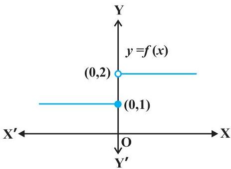 Fig 5.1
Expressed in terms of limits, the left-hand limit of $f$ at 0 is 1, while its right-hand limit at 0 is 2. Crucially, these one-sided limits are not equal. Furthermore, we note that the function's value at $x = 0$ corresponds to its left-hand limit. Graphically, this characteristic implies that the function's curve cannot be traced in a single continuous motion; one must lift the pen when transitioning across $x = 0$. This exemplifies a function that lacks continuity at $x = 0$.
Next, let us examine the function defined as follows:
$ f (x) = \left{ \begin{array}{l} 1, \text { if } x \neq 0 \ 2, \text { if } x = 0 \end{array} \right. $
This function, too, possesses a defined value at every point on the real axis. At $x = 0$, both the left-hand
and right-hand limits converge to 1. However, the function's actual value at $x = 0$ is 2, which diverges from this common limit. Once more, its graph cannot be drawn without lifting the pen, thereby illustrating another scenario where a function is discontinuous at $x = 0$.
Intuitively, a function can be deemed continuous at a specific point if its graph can be sketched in the vicinity of that point without detaching the writing instrument from the surface.
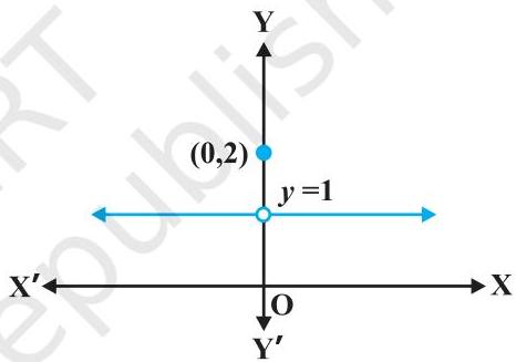 Fig 5.2
From a mathematical perspective, this concept is formally defined as follows:
Definition 1 Suppose $f$ is a real function on a subset of the real numbers and let $c$ be a point in the domain of $f$. Then $f$ is continuous at $c$ if
$ \lim _ {x \rightarrow c} f (x) = f (c) $
To elaborate, a function $f$ is considered continuous at $x = c$ if its left-hand limit, right-hand limit, and its actual value at $x = c$ all exist and are mutually equivalent. It is pertinent to recall that when the right-hand and left-hand limits at $x = c$ converge to the same value, this shared value constitutes the overall limit of the function at $x = c$. Consequently, an alternative formulation for the definition of continuity states that a function is continuous at $x = c$ if it is defined at $x = c$
and its value at $x = c$ is identical to its limit at $x = c$. Should $f$ fail to be continuous at $c$, it is termed discontinuous at $c$, and $c$ is designated as a point of discontinuity for $f$.
Example 1 Determine if the function $f$ given by $f(x) = 2x + 3$ is continuous at $x = 1$.
Solution Initially, observe that the function is well-defined at the specified point $x = 1$, with a corresponding value of 5. Subsequently, ascertain the limit of the function as $x$ approaches 1. Evidently,
$ \lim_{x \to 1} f(x) = \lim_{x \to 1} (2x + 3) = 2(1) + 3 = 5 $
Consequently,
$ \lim_{x \to 1} f(x) = 5 = f(1) $
Therefore, the function $f$ exhibits continuity at $x = 1$.
Example 2 Investigate the continuity of the function $f$ given by $f(x) = x^2$ at $x = 0$.
Solution Initially, observe that the function is well-defined at the specified point $x = 0$, where its value is 0. Next, determine the limit of the function as $x$ approaches 0. It is evident that
$ \lim_{x \to 0} f(x) = \lim_{x \to 0} x^2 = 0^2 = 0 $
Hence,
$ \lim_{x \to 0} f(x) = 0 = f(0) $
Consequently, $f$ is continuous at $x = 0$.
Example 3 Analyze the continuity of the function $f$ given by $f(x) = |x|$ at $x = 0$.
Solution As defined,
$ f(x) = \begin{cases} -x, & \text{if } x \leq 0 \ x, & \text{if } x \geq 0 \end{cases} $
It is clear that the function is defined at 0, with $f(0) = 0$. The left-hand limit of $f$ as $x$ approaches 0 is
$ \lim_{x \to 0^-} f(x) = \lim_{x \to 0^-} (-x) = 0 $
Likewise, the right-hand limit of $f$ as $x$ approaches 0 is
$ \lim_{x \to 0^+} f(x) = \lim_{x \to 0^+} x = 0 $
Consequently, the left-hand limit, the right-hand limit, and the function's value all converge at $x = 0$. Therefore, $f$ demonstrates continuity at $x = 0$.
Example 4 Demonstrate that the function $f$ given by
$ f(x) = \begin{cases} x^3 + 3, & \text{if } x \neq 0 \ 1, & \text{if } x = 0 \end{cases} $
lacks continuity at $x = 0$.
Solution The function is well-defined at $x = 0$, where its value is 1. For $x \neq 0$, the function's expression is that of a polynomial. Consequently,
$ \lim_{x \to 0} f(x) = \lim_{x \to 0} (x^3 + 3) = 0^3 + 3 = 3 $
As the limit of $f$ as $x$ approaches 0 does not equate to $f(0)$, the function is not continuous at $x = 0
$. It is worth observing that $x = 0$ constitutes the sole point of discontinuity for this function.
Example 5 Determine the domain of continuity for the constant function $f(x) = k$.
Solution The function is defined across all real numbers, and by its definition, its value at any real number is $k$. Consider an arbitrary real number, $c$. In this case,
$ \lim_{x \to c} f(x) = \lim_{x \to c} k = k $
Given that $f(c) = k = \lim_{x \to c} f(x)$ for any real number $c$, the function $f$ is continuous throughout the entire set of real numbers.
Example 6 Demonstrate that the identity function defined on real numbers as $f(x) = x$ exhibits continuity across all real numbers.
Solution The function is unequivocally defined at each point, with $f(c) = c$ for any real number $c$. Furthermore,
$ \lim_{x \to c} f(x) = \lim_{x \to c} x = c $
Consequently, as $\lim_{x \to c} f(x) = c = f(c)$, the function is continuous for all real numbers.
Following the establishment of a function's continuity at a specific point, we now proceed to a logical extension of this definition to encompass the continuity of a function more broadly.
Definition 2 A real function $f$ is considered continuous if it maintains continuity at every single point within its designated domain.
This particular definition necessitates some further explanation. Consider a function $f$ whose domain is the closed interval $[a, b]$. For $f$ to be deemed continuous across this interval, it must exhibit continuity at every single point within $[a, b]$, including its boundary points, $a$ and $b$. The condition for $f$ to be continuous at point $a$ is articulated as:
$ \lim_{x \to a^-} f(x) = f(a) $
Similarly, the criterion for $f$ to be continuous at point $b$ is expressed as:
$ \lim_{x \to b^-} f(x) = f(b) $
It is important to recognize that the expressions $\lim_{x \to a^-} f(x)$ and $\lim_{x \to b^-} f(x)$ are not meaningful in this context. Consequently, an implication of this definition is that if a function $f$ is defined solely at a single point, it is considered continuous at that point; in other words, if the domain of $f$ comprises a solitary element, then $f$ is a continuous function.
Example 7 Determine whether the function specified by $f(x) = |x|$ exhibits continuity.
Solution The function $f$ can be expressed in an alternative form as follows:
$ f(x) = \begin{cases} -x, & \text{if } x < 0 \ x, & \text{if } x \geq 0 \end{cases} $
As established in Example 3, the function $f$ maintains continuity at $x = 0$.
Consider an arbitrary real number $c$ such that $c < 0$. In this case, $f(c) = -c$. Furthermore,
$ \lim_{x \to c} f(x) = \lim_{x \to c} (-x) = -c \quad \text{(Why?)} $
Given that $\lim_{x \to c} f(x) = f(c)$, it follows that $f$ is continuous across all negative real numbers.
Next, let $c$ be a real number satisfying $c > 0$. Here, $f(c) = c$. Additionally,
$ \lim_{x \to c} f(x) = \lim_{x \to c} x = c \quad \text{(Why?)} $
Because $\lim_{x \to c} f(x) = f(c)$, $f$ demonstrates continuity for all positive real numbers. Consequently, $f$ is continuous at every point in its domain.
Example 8 Examine the continuity of the function $f$ defined as $f(x) = x^3 + x^2 - 1$.
Solution It is evident that $f$ is defined for every real number $c$, and its corresponding value at $c$ is $c^3 + c^2 - 1$. We are also aware that
$ \lim_{x \to c} f(x) = \lim_{x \to c} (x^3 + x^2 - 1) = c^3 + c^2 - 1 $
Therefore, $\lim_{x \to c} f(x) = f(c)$, which implies that $f$ is continuous at every real number. This establishes $f$ as a continuous function.
Example 9 Investigate the continuity of the function $f$ given by $f(x) = \frac{1}{x}, x \neq 0$.
Solution For any arbitrary non-zero real number $c$, we obtain:
$ \lim_{x \to c} f(x) = \lim_{x \to c} \frac{1}{x} = \frac{1}{c} $
Moreover, since $f(c) = \frac{1}{c}$ for $c \neq 0$, it follows that $\lim_{x \to c} f(x) = f(c)$. Consequently, $f$ is continuous at every point within its domain. Hence, $f$ is a continuous function.
We shall utilize this juncture to elucidate the notion of infinity. Our approach involves examining the behavior of the function $f(x) = \frac{1}{x}$ in the vicinity of $x = 0$. To conduct this examination,
we employ the conventional method of evaluating the function's value at real numbers arbitrarily close to 0. Fundamentally, our objective is to ascertain the right-hand limit of $f$ at 0. This is presented in tabular form below (Table 5.1).
Table 5.1
| x | 1 | 0.3 | 0.2 | 0.1 = 10⁻¹ | 0.01 = 10⁻² | 0.001 = 10⁻³ | 10⁻ⁿ |
|---|---|---|---|---|---|---|---|
| f(x) | 1 | 3.333... | 5 | 10 | 100 = 10² | 1000 = 10³ | 10ⁿ |
It is discernible that as $x$ approaches 0 from the positive side, the corresponding value of $f(x)$ increases without bound. This phenomenon can be restated as: the magnitude of $f(x)$ can be made to exceed any specified number by selecting a positive real number sufficiently close to 0. Symbolically, this is expressed as:
$ \lim _ {x \rightarrow 0 ^ {+}} f (x) = + \infty $
(to be interpreted as: the right-sided limit of $f(x)$ as $x$ approaches $0$ from the positive direction is positive infinity). It is imperative to underscore that $+\infty$ does NOT represent a real number; consequently, the right-sided limit of $f$ at $0$ does not exist (within the set of real numbers).
The determination of the left-sided limit of $f$ at $0$ can be performed similarly. Table 5.2 provides a clear illustration.
Table 5.2
| x | −1 | −0.3 | −0.2 | −10⁻¹ | −10⁻² | −10⁻³ | −10⁻ⁿ |
|---|---|---|---|---|---|---|---|
| f(x) | −1 | −3.333... | −5 | −10 | −10² | −10³ | −10ⁿ |
Analysis of Table 5.2 reveals that the value of $f(x)$ can be rendered arbitrarily small by selecting a negative real number in close proximity to zero. Symbolically, we express this as
$ \lim _ {x \rightarrow 0 ^ {-}} f (x) = - \infty $
(to be interpreted as: the left-sided limit of $f(x)$ as $x$ approaches $0$ from the negative direction is negative infinity). It is crucial to reiterate that $-\infty$ is NOT a real number, and therefore, the left-sided limit of $f$ at $0$ does not exist (as a real number). The accompanying graph of the reciprocal function, presented in Fig 5.3, offers a visual depiction of these observations.
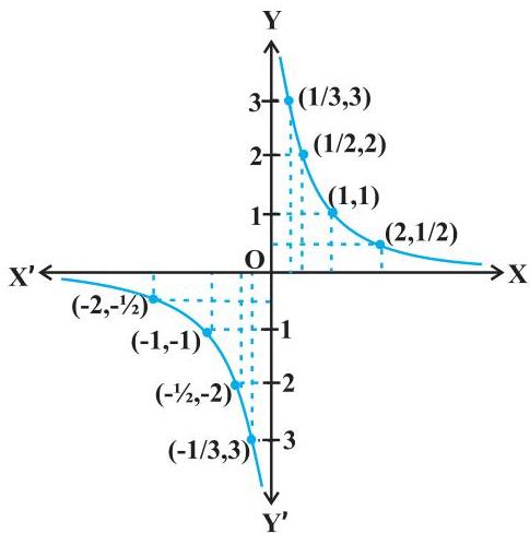 Fig 5.3
Example 10 Examine the continuity properties of the function $f$ as defined by
$ f(x) = \begin{cases} x + 2, & \text{if } x \leq 1 \ x - 2, & \text{if } x > 1 \end{cases} $
Solution The domain of function $f$ encompasses the entirety of the real number line.
Case 1 For any $c < 1$, the function value $f(c)$ is $c + 2$. Consequently, the limit as $x$ approaches $c$ for $f(x)$ is $\lim_{x \to c} (x + 2)$, which evaluates to $c + 2$.
Hence, $f$ exhibits continuity across all real numbers strictly less than 1.
Case 2 For any $c > 1$, the function value $f(c)$ is $c - 2$. Accordingly,
$ \lim_{x \to c} f(x) = \lim_{x \to c} (x - 2) = c - 2 = f(c) $
Therefore, $f$ is continuous at all points where $x > 1$.
Case 3 When $c = 1$, the left-sided limit of $f$ as $x$ approaches $1$ is determined as
$ \lim_{x \to 1^{-}} f(x) = \lim_{x \to 1^{-}} (x + 2) = 1 + 2 = 3 $
Conversely, the right-sided limit of $f$ as $x$ approaches $1$ is calculated as
$ \lim_{x \to 1^{+}} f(x) = \lim_{x \to 1^{+}} (x - 2) = 1 - 2 = -1 $
As the left-sided and right-sided limits of $f$ at $x = 1$ are unequal, the function $f$ is discontinuous at $x = 1$. Therefore, $x = 1$ represents the sole point of discontinuity for $f$. Fig 5.4 illustrates the graphical representation of this function.
Example 11 Identify all points of discontinuity for the function $f$ defined as
$ f(x) = \begin{cases} x + 2, & \text{if } x < 1 \ 0, & \text{if } x = 1 \ x - 2, & \text{if } x > 1 \end{cases} $
Solution Consistent with the preceding example, it is observed that $f$ maintains continuity across all real numbers except $x = 1$. At $x = 1$, the left-sided limit of $f$ is given by
$ \lim_{x \to 1^{-}} f(x) = \lim_{x \to 1^{-}} (x + 2) = 1 + 2 = 3 $
Conversely, the right-sided limit of $f$ at $x = 1$ is determined as
$ \lim_{x \to 1^{+}} f(x) = \lim_{x \to 1^{+}} (x - 2) = 1 - 2 = -1 $
Given that the left-sided and right-sided limits of $f$ at $x = 1$ are divergent, the function $f$ is discontinuous at $x = 1$. Consequently, $x = 1$ constitutes the sole point of discontinuity for $f$. The graphical representation of this function is provided in Fig 5.5.
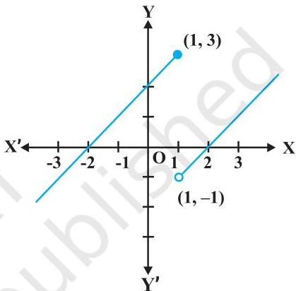 Fig 5.4
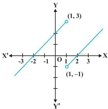 Fig 5.5
Example 12 Examine the continuity of the function specified as:
$ f(x) = \begin{cases} x + 2, & \text{if } x < 0 \ -x + 2, & \text{if } x > 0 \end{cases} $
Solution It is apparent that this function is defined for all real numbers, with the exception of 0. The domain of definition for this function comprises:
$\mathrm{D}_1 \cup \mathrm{D}_2$ where $\mathrm{D}_1 = {x \in \mathbf{R} : x < 0}$ and
$\mathrm{D}_2 = {x \in \mathbf{R} : x > 0}$
Case 1 For any $c$ belonging to $\mathrm{D}1$, the limit of $f(x)$ as $x$ approaches $c$ is given by $\lim{x \to c} f(x) = \lim_{x \to c} (x + 2)$
$= c + 2 = f(c)$, thereby establishing that $f$ is continuous throughout $\mathrm{D}_1$.
Case 2 Similarly, if $c \in \mathrm{D}2$, then the limit $\lim{x \to c} f(x)$ evaluates to $\lim_{x \to c} (-x + 2)$
$= -c + 2 = f(c)$, which demonstrates $f
YoLearn.AI is India's #1 AI tutoring platform for Class 1 to 12, JEE, and NEET preparation.
Students talk to expert AI tutors in real time through live voice calls, solve doubts instantly
on an interactive sketch board, and practice with mock tests, flashcards, quizzes, and slide decks.
Learn from top educators including DC Pandey and other verified teachers who create AI avatars of themselves.
Unlike text-only chatbots, YoLearn.AI lets you speak naturally to your AI tutor — just like a real
one-on-one session. Get step-by-step explanations for Physics, Chemistry, Maths, and Biology
for board exams, JEE Main, JEE Advanced, and NEET.
Prepare for JEE 2026, NEET 2026, and CBSE board exams with personalized mock tests, AI-generated
quizzes, and flashcard makers. Build daily study habits with an AI study buddy designed for Indian students.
Whether you need a Class 10 CBSE tutor, Class 12 board exam help, or full JEE and NEET coaching online,
YoLearn.AI adapts to your grade, syllabus, and learning pace. Start free today on web, iOS, and Android.
Personal 1:1 AI Tutor for CBSE, JEE & NEET Students
Live voice tutoring and doubt solving
Mock tests, flashcards, and exam prep
For school, JEE, and NEET
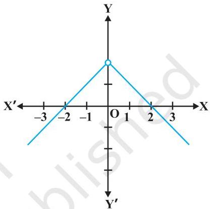 Fig 5.6
Example 13 Analyze the continuity of the function $f$ defined as:
$ f(x) = \begin{cases} x, & \text{if } x \geq 0 \ x^2, & \text{if } x < 0 \end{cases} $
Solution This function is evidently defined for all real numbers. Its graph is illustrated in Fig 5.7. A preliminary examination suggests that it would be judicious to segment the function's domain into three mutually exclusive subsets of the real number line.
Let $\mathrm{D}_1 = {x \in \mathbf{R} : x < 0}, \mathrm{D}_2 = {0}$ and $\mathrm{D}_3 = {x \in \mathbf{R} : x > 0}$
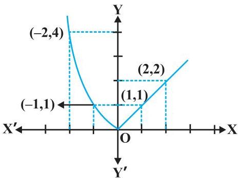 Fig 5.7
Case 1 For any point within $\mathrm{D}_1$, the function is expressed as $f(x) = x^2$, which is readily identifiable as continuous in this region (refer to Example 2).
Case 2 Similarly, for any point in $\mathrm{D}_3$, $f(x) = x$, and its continuity in this interval is straightforward to ascertain (refer to Example 6).
Case 3 The behavior of the function at $x = 0$ is now examined. The functional value at 0 is $f(0) = 0$. The limit of $f$ from the left as $x$ approaches 0 is:
$ \lim_{x \to 0^{-}} f(x) = \lim_{x \to 0^{-}} x^{2} = 0^{2} = 0 $
Conversely, the limit of $f$ from the right as $x$ approaches 0 is:
$ \lim_{x \to 0^{+}} f(x) = \lim_{x \to 0^{+}} x = 0 $
Consequently, $\lim_{x\to 0}f(x) = 0 = f(0)$, which confirms $f
YoLearn.AI is India's #1 AI tutoring platform for Class 1 to 12, JEE, and NEET preparation.
Students talk to expert AI tutors in real time through live voice calls, solve doubts instantly
on an interactive sketch board, and practice with mock tests, flashcards, quizzes, and slide decks.
Learn from top educators including DC Pandey and other verified teachers who create AI avatars of themselves.
Unlike text-only chatbots, YoLearn.AI lets you speak naturally to your AI tutor — just like a real
one-on-one session. Get step-by-step explanations for Physics, Chemistry, Maths, and Biology
for board exams, JEE Main, JEE Advanced, and NEET.
Prepare for JEE 2026, NEET 2026, and CBSE board exams with personalized mock tests, AI-generated
quizzes, and flashcard makers. Build daily study habits with an AI study buddy designed for Indian students.
Whether you need a Class 10 CBSE tutor, Class 12 board exam help, or full JEE and NEET coaching online,
YoLearn.AI adapts to your grade, syllabus, and learning pace. Start free today on web, iOS, and Android.
Personal 1:1 AI Tutor for CBSE, JEE & NEET Students
Live voice tutoring and doubt solving
Mock tests, flashcards, and exam prep
For school, JEE, and NEET
Example 14 Demonstrate the continuity of any polynomial function.
Solution It is important to remember that a function $p$ is characterized as a polynomial if its definition is given by $p(x) = a_0 + a_1 x + \ldots + a_n x^n$, where $n$ is a natural number, $a_n \neq 0$, and each $a_i \in \mathbf{R}$. This function is self-evidently defined for all real numbers. Considering an arbitrary, fixed real number $c$, we possess:
$ \lim_{x \to c} p(x) = p(c) $
This relationship, by its very definition, establishes the continuity of $p$ at point $c$. Given that $c$ represents an arbitrary real number, it follows that $p$ exhibits continuity across the entire set of real numbers, thereby classifying $p$ as a continuous function.
Example 15 Determine the complete set of discontinuity points for the greatest integer function, denoted as $f(x) = [x]$, where $[x]$ signifies the largest integer that is less than or equal to $x$.
Solution Initially, we note that the function $f$ possesses a domain encompassing all real numbers. The graphical representation of this function is provided in Fig 5.8. An initial visual inspection of the graph suggests that $f$ might exhibit discontinuities at each integer value. We will now proceed to rigorously investigate this preliminary observation.
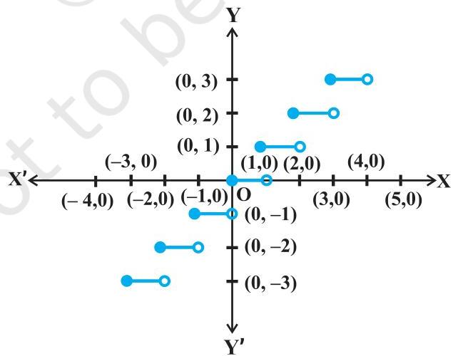 Fig 5.8
Case 1 Consider an arbitrary real number $c$ that is not an integer. From the graphical depiction, it becomes apparent that for any real numbers in the immediate vicinity of $c$, the function's output remains constant and equal to $[c]$. This implies that $\lim_{x \to c} f(x) = \lim_{x \to c} [x] = [c]$. Furthermore, the function's value at $c$ is $f(c) = [c]$. Consequently, the function demonstrates continuity at all real numbers that are not integers.
Case 2 Now, let $c$ be an integer. In this scenario, it is possible to select a sufficiently small positive real number $r$ such that the greatest integer less than or equal to $c - r$ is $c - 1$, while the greatest integer less than or equal to $c + r$ is $c$.
Expressed using the concept of limits, this observation means that:
$ \lim_{x \to c^{-}} f(x) = c - 1, \quad \lim_{x \to c^{+}} f(x) = c $
Given that the left-hand limit and the right-hand limit are inherently unequal for
any integer $c$, the function fails to be continuous at every integral point.
5.2.1 Algebra of continuous functions
Having previously established the algebraic properties of limits following an understanding of their fundamental concept, we now turn our attention to the corresponding algebra of continuous functions. Given that the continuity of a function at a specific point is entirely determined by its limit at that point, it logically follows that we can anticipate analogous outcomes to those observed for limits.
Theorem 1 Let $f$ and $g$ represent two real-valued functions that are continuous at a real number $c$. Then the following hold:
(1) $f + g$ is continuous at $x = c$.
(2) $f - g$ is continuous at $x = c$.
(3) $f \cdot g$ is continuous at $x = c$.
(4) $\left(\frac{f}{g}\right)$ is continuous at $x = c$, (provided $g(c) \neq 0$).
Proof Our objective is to ascertain the continuity of the sum function $(f + g)$ at the point $x = c$. It is evident that this function is well-defined at $x = c$. We proceed as follows:
$ \begin{array}{l} \lim_{x \to c} (f + g)(x) = \lim_{x \to c} [f(x) + g(x)] \quad (\text{by definition of } f + g) \ = \lim_{x \to c} f(x) + \lim_{x \to c} g(x) \quad (\text{by the theorem on limits}) \ = f(c) + g(c) \quad (\text{as } f \text{ and } g \text{ are continuous}) \ = (f + g)(c) \quad (\text{by definition of } f + g) \end{array} $
Consequently, it is established that $f + g$ maintains continuity at $x = c$.
The demonstrations for the remaining assertions are structurally analogous and are therefore provided as an exercise for the reader.
Remarks
(i) Considering (3) as a specific instance, when $f$ represents a constant function, specifically $f(x) = \lambda$ for some real number $\lambda$, it follows that the function $(\lambda \cdot g)$, articulated as $(\lambda \cdot g)(x) = \lambda \cdot g(x)$, also exhibits continuity. Notably, if $\lambda$ takes the value $-1$, the continuous nature of $f$ guarantees the continuity of $-f$.
(ii) By applying (4) as a particular scenario, if $f$ is the constant function $f(x) = \lambda$, then the function $\frac{\lambda}{g}$, defined by $\frac{\lambda}{g}(x) = \frac{\lambda}{g(x)}$, similarly maintains continuity wherever $g(x) \neq 0$. In particular, the continuity of $g$ directly implies the continuity of $\frac{1}{g}$.
The aforementioned theorem offers a means to construct numerous continuous functions. Furthermore, it assists in determining whether specific functions possess continuity. The subsequent examples serve to elucidate this principle:
Example 16 Prove that every rational function is continuous.
Solution It is known that any rational function $f$ is expressed as
$ f(x) = \frac{p(x)}{q(x)}, \quad q(x) \neq 0 $
where $p$ and $q$ denote polynomial expressions. The function $f
YoLearn.AI is India's #1 AI tutoring platform for Class 1 to 12, JEE, and NEET preparation.
Students talk to expert AI tutors in real time through live voice calls, solve doubts instantly
on an interactive sketch board, and practice with mock tests, flashcards, quizzes, and slide decks.
Learn from top educators including DC Pandey and other verified teachers who create AI avatars of themselves.
Unlike text-only chatbots, YoLearn.AI lets you speak naturally to your AI tutor — just like a real
one-on-one session. Get step-by-step explanations for Physics, Chemistry, Maths, and Biology
for board exams, JEE Main, JEE Advanced, and NEET.
Prepare for JEE 2026, NEET 2026, and CBSE board exams with personalized mock tests, AI-generated
quizzes, and flashcard makers. Build daily study habits with an AI study buddy designed for Indian students.
Whether you need a Class 10 CBSE tutor, Class 12 board exam help, or full JEE and NEET coaching online,
YoLearn.AI adapts to your grade, syllabus, and learning pace. Start free today on web, iOS, and Android.
Personal 1:1 AI Tutor for CBSE, JEE & NEET Students
Live voice tutoring and doubt solving
Mock tests, flashcards, and exam prep
For school, JEE, and NEET
Example 17 Discuss the continuity of sine function.
Solution To demonstrate this, we employ the subsequent established facts:
$ \lim_{x \to 0} \sin x = 0 $
While not formally proven here, this assertion is intuitively evident upon examining the graph of $\sin x$ in the vicinity of 0.
Next, it can be observed that the function $f(x) = \sin x$ holds a defined value for all real numbers. Consider an arbitrary real number $c$. Let $x$ be expressed as $c + h$. As $x$ approaches $c$, it follows that $h$ approaches $0$. Consequently,
$ \begin{aligned} \lim_{x \to c} f(x) &= \lim_{x \to c} \sin x \ &= \lim_{h \to 0} \sin(c + h) \ &= \lim_{h \to 0} [\sin c \cos h + \cos c \sin h] \ &= \lim_{h \to 0} [\sin c \cos h] + \lim_{h \to 0} [\cos c \sin h] \ &= \sin c + 0 = \sin c = f(c) \end{aligned} $
Consequently, since $\lim_{x \to c} f(x) = f(c)$, the function $f$ is therefore continuous.
Remark: An analogous proof can be constructed to establish the continuity of the cosine function.
Example 18 Prove that the function defined by $f(x) = \tan x$ is a continuous function.
Solution The function $f(x) = \tan x$ is equivalently expressed as $\frac{\sin x}{\cos x}$. Its domain includes all real numbers for which $\cos x$ is non-zero, which means $x \neq (2n + 1)\frac{\pi}{2}$. As previously demonstrated, both the sine and cosine functions exhibit continuity. Therefore, $\tan x$, being the ratio of two continuous functions, maintains continuity across its entire domain of definition.
A notable aspect concerns how continuous functions behave under the operation of function composition. It should be remembered that for any two real functions $f$ and $g$,
$ (f \circ g) (x) = f (g (x)) $
this composite is defined provided the range of $g$ is contained within the domain of $f$. The ensuing theorem (presented without formal derivation) delineates the continuity properties of composite functions.
Theorem 2 Suppose $f$ and $g$ are real valued functions such that $(f \circ g)$ is defined at $c$. If $g$ is continuous at $c$ and if $f$ is continuous at $g(c)$, then $(f \circ g)$ is continuous at $c$.
The following examples illustrate this theorem.
Example 19 Demonstrate the continuity of the function $f(x) = \sin (x^2)$.
Solution It is evident that the function's domain encompasses all real numbers. The function $f$ can be conceptualized as the composition $g \circ h$ of two distinct functions: $g(x) = \sin x$ and $h(x) = x^2$. Given that both $g$ and $h$ are continuous functions, it logically follows from Theorem 2 that $f$ is also a continuous function.
Example 20 Establish the continuity of the function $f$ given by
$ f (x) = | 1 - x + | x | |, $
for all real numbers $x$.
Solution Let us define two functions: $g(x) = 1 - x + |x|$ and $h(x) = |x|$, applicable for all real $x$. Subsequently, the composition $(h \circ g)(x)$ yields:
$ \begin{array}{l} (h \circ g) (x) = h (g (x)) \ = h (1 - x + | x |) \ = | 1 - x + | x | | = f (x) \end{array} $
From Example 7, it is established that $h$ is a continuous function. Furthermore, $g$ is continuous because it represents the sum of a polynomial function and the absolute value function, both of which are continuous. Consequently, since $f$ is formed by the composition of two continuous functions, $f$ itself must be continuous.
EXERCISE 5.1
Demonstrate the continuity of the function $f(x) = 5x - 3$ at the specific points $x = 0$, $x = -3$, and $x = 5$.
Investigate the continuity of the function $f(x) = 2x^{2} - 1$ at the point $x = 3$.
Evaluate the continuity of the subsequent functions.
(a) $f(x) = x - 5$
(b) $f(x) = \frac{1}{x - 5}, x \neq 5$
(c) $f(x) = \frac{x^2 - 25}{x + 5}, x \neq -5$
(d) $f(x) = |x - 5|$
Establish the continuity of the function $f(x) = x^{n}$ at $x = n$, given that $n$ is a positive integer.
Consider the function $f$ specified by
$ f(x) = \begin{cases} x, & \text{if } x \leq 1 \ 5, & \text{if } x > 1 \end{cases} $
Determine if it is continuous at $x = 0$, at $x = 1$, and at $x = 2$.
Identify every point of discontinuity for the function $f$, as defined below.
6.[ f(x)= \begin{cases} 2x+3, & \text{if } x\le 2 \ 2x-3, & \text{if } x>2 \end{cases} ]
7.[ f(x)= \begin{cases} |x|+3, & \text{if } x\le -3 \ -2x, & \text{if } -3<x<3 \ 6x+2, & \text{if } x\ge 3 \end{cases} ]
8.[ f(x)= \begin{cases} \dfrac{|x|}{x}, & \text{if } x\ne 0 \ 0, & \text{if } x=0 \end{cases} ]
9.[ f(x)= \begin{cases} \dfrac{x}{|x|}, & \text{if } x<0 \ -1, & \text{if } x\ge 0 \end{cases} ]
10.[ f(x)= \begin{cases} x+1, & \text{if } x\ge 1 \ x^2+1, & \text{if } x<1 \end{cases} ]
11.[ f(x)= \begin{cases} x^3-3, & \text{if } x\le 2 \ x^2+1, & \text{if } x>2 \end{cases} ]
12.[ f(x)= \begin{cases} x^{10}-1, & \text{if } x\le 1 \ x^2, & \text{if } x>1 \end{cases} ]
- For the function (f) given by
[ f(x)= \begin{cases} x+5, & \text{if } x\le 1 \ x-5, & \text{if } x>1 \end{cases} ]
ascertain whether it is a continuous function.
Analyze the continuity of the function $f$, as specified by its definition below.
14.[ f(x)= \begin{cases} 3, & \text{if } 0\le x\le 1 \ 4, & \text{if } 1<x<3 \ 5, & \text{if } 3\le x\le 10 \end{cases} ]
15.[ f(x)= \begin{cases} 2x, & \text{if } x<0 \ 0, & \text{if } 0\le x\le 1 \ 4x, & \text{if } x>1 \end{cases} ]
16.[ f(x)= \begin{cases} -2, & \text{if } x\le -1 \ 2x, & \text{if } -1<x\le 1 \ 2, & \text{if } x>1 \end{cases} ]
- Determine the requisite relationship between the constants (a) and (b) such that the function (f), defined as
[ f(x)= \begin{cases} ax+1, & \text{if } x\le 3 \ bx+3, & \text{if } x>3 \end{cases} ]
maintains continuity at the point (x=3).
- For what specific value of (\lambda) does the function, expressed as
[ f(x)= \begin{cases} \lambda(x^2-2x), & \text{if } x\le 0 \ 4x+1, & \text{if } x>0 \end{cases} ]
exhibit continuity at (x=0)? Furthermore, consider its continuity at (x=1).
- Demonstrate that the function
[ g(x)=x-[x] ]
is discontinuous across all integral points. In this context, ([x]) represents the greatest integer less than or equal to (x).
- Ascertain whether the function
[ f(x)=x^2-\sin x+5 ]
is continuous at the point (x=\pi).
- Analyze the continuity of the subsequent functions:
(a) $f(x) = \sin x + \cos x$
(b) $f(x) = \sin x - \cos x$
(c) $f(x) = \sin x \cdot \cos x$
Analyze the continuity properties of the cosine, cosecant, secant, and cotangent functions.
Identify all points of discontinuity for the function $f$, where $f$ is defined as:
$ f(x) = \begin{cases} \frac{\sin x}{x}, & \text{if } x < 0 \ x + 1, & \text{if } x \geq 0 \end{cases} $
- Ascertain whether the function $f$, defined by the expression:
$ f(x) = \begin{cases} x^2 \sin \frac{1}{x}, & \text{if } x \neq 0 \ 0, & \text{if } x = 0 \end{cases} $
is continuous.
- Investigate the continuity of the function $f$, which is specified by:
$ f(x) = \begin{cases} \sin x - \cos x, & \text{if } x \neq 0 \ -1, & \text{if } x = 0 \end{cases} $
For Exercises 26 through 29, determine the values of $k$ such that the function $f$ maintains continuity at the designated point.
- $ f(x) = \begin{cases} \dfrac{k\cos x}{\pi - 2x}, & \text{if } x \neq \dfrac{\pi}{2} \ 3, & \text{if } x = \dfrac{\pi}{2} \end{cases} \text{ at } x = \dfrac{\pi}{2} $
27.[ f(x)= \begin{cases} kx^2, & \text{if } x\le 2 \ 3, & \text{if } x>2 \end{cases} \quad \text
{at } x=2 ]
28.[ f(x)= \begin{cases} kx+1, & \text{if } x\le \pi \ \cos x, & \text{if } x>\pi \end{cases} \quad \text{at } x=\pi ]
29.[ f(x)= \begin{cases} kx+1, & \text{if } x\le 5 \ 3x-5, & \text{if } x>5 \end{cases} \quad \text{at } x=5 ]
- Ascertain the values of $a$ and $b$ for which the function $f$, defined as:
$ f(x) = \begin{cases} 5, & \text{if } x \leq 2 \ ax + b, & \text{if } 2 < x < 10 \ 21, & \text{if } x \geq 10 \end{cases} $
is continuous across its entire domain.
Demonstrate that the function $f(x) = \cos(x^2)$ is continuous.
Prove the continuity of the function $f(x) = |\cos x|$.
Investigate whether $\sin |x|$ constitutes a continuous function.
Identify every point where the function $f$, defined by $f(x) = |x| - |x + 1|$, exhibits discontinuity.
5.3. Differentiability
Let us review key concepts from prior lessons. The derivative of a real-valued function was previously defined as follows:
Given a real function $f$ and a point $c$ within its domain, the derivative of $f$ evaluated at $c$ is formally expressed as:
$ \lim_{h \to 0} \frac{f(c + h) - f(c)}{h} $
This definition holds true provided the limit exists. The derivative of $f$ at point $c$ is commonly represented by $f'(c)$ or $\left. \frac{d}{dx} (f(x)) \right|_c$. Furthermore, the function derived from this process, given by
$ f^{\prime}(x) = \lim_{h \rightarrow 0} \frac{f(x + h) - f(x)}{h} $
wherever this limit converges, is termed the derivative of $f$. This derivative is commonly symbolized as $f'(x)$, $\frac{d}{dx} (f(x))$, or, if $y = f(x)$, as $\frac{dy}{dx}$ or $y'$. The procedure for determining a function's derivative is known as differentiation. The instruction to 'differentiate $f(x)$ with respect to $x
YoLearn.AI is India's #1 AI tutoring platform for Class 1 to 12, JEE, and NEET preparation.
Students talk to expert AI tutors in real time through live voice calls, solve doubts instantly
on an interactive sketch board, and practice with mock tests, flashcards, quizzes, and slide decks.
Learn from top educators including DC Pandey and other verified teachers who create AI avatars of themselves.
Unlike text-only chatbots, YoLearn.AI lets you speak naturally to your AI tutor — just like a real
one-on-one session. Get step-by-step explanations for Physics, Chemistry, Maths, and Biology
for board exams, JEE Main, JEE Advanced, and NEET.
Prepare for JEE 2026, NEET 2026, and CBSE board exams with personalized mock tests, AI-generated
quizzes, and flashcard makers. Build daily study habits with an AI study buddy designed for Indian students.
Whether you need a Class 10 CBSE tutor, Class 12 board exam help, or full JEE and NEET coaching online,
YoLearn.AI adapts to your grade, syllabus, and learning pace. Start free today on web, iOS, and Android.
Personal 1:1 AI Tutor for CBSE, JEE & NEET Students
Live voice tutoring and doubt solving
Mock tests, flashcards, and exam prep
For school, JEE, and NEET
The subsequent rules were previously established as fundamental components of the algebra of derivatives:
(1) $(u\pm v)' = u'\pm v'$ (2) $(uv)' = u'v + uv'$ (Leibnitz or product rule) (3) $\left(\frac{u}{v}\right)' = \frac{u'v - uv'}{v^2}$ , wherever $v \neq 0$ (Quotient rule).
The table presented below enumerates the derivatives of several standard functions:
Table 5.3
| f(x) | xⁿ | sin x | cos x | tan x |
|---|---|---|---|---|
| f′(x) | n xⁿ⁻¹ | cos x | −sin x | sec² x |
When the derivative was initially defined, a crucial caveat was included: the existence of the limit. This naturally prompts the inquiry: what occurs if the limit fails to exist? This question is highly relevant, and its resolution is equally clear. Should the limit $\lim_{h\to 0}\frac{f(c + h) - f(c)}{h}$ not exist, we assert that $f$ is not differentiable at $c$. Stated differently, a function $f$ is considered differentiable at a point $c$ within its domain if both the right-hand limit $\lim_{h\to 0^+}\frac{f(c + h) - f(c)}{h}$ and the left-hand limit $\lim_{h\to 0^-}\frac{f(c + h) - f(c)}{h}$ are finite and yield identical values. A function is deemed differentiable over a closed interval $[a,b]$ if it exhibits differentiability at every point within that interval. Analogous to the definition of continuity, at the interval's endpoints, $a$ and $b$, we consider the right-hand limit and left-hand limit, respectively, which correspond to the right-hand derivative and left-hand derivative of the function at $a$ and $b$. Likewise, a function is said to be differentiable across an open interval $(a,b)$ if it is differentiable at every point within that interval.
Theorem 3: If a function $f$ possesses differentiability at a specific point $c$, then it necessarily follows that the function is also continuous at that same point.
Proof: Given that $f$ is differentiable at $c$, it implies that:
$ \lim_{x \to c} \frac{f(x) - f(c)}{x - c} = f'(c) $
However, for any $x$ distinct from $c$, we can write:
$ f(x) - f(c) = \frac{f(x) - f(c)}{x - c} \cdot (x - c) $
Consequently, applying the limit as $x$ approaches $c$ to both sides yields:
$ \lim_{x\to c}[f(x) - f(c)] = \lim_{x\to c}\left[\frac{f(x) - f(c)}{x - c} \cdot (x - c)\right] $
This can be expanded as:
$ \lim_{x\to c}[f(x)] - \lim_{x\to c}[f(c)] = \lim_{x\to c}\left[\frac{f(x) - f(c)}{x - c}\right] \cdot \lim_{x\to c}[(x - c)] $
$ = f'(c) \cdot 0 = 0 $
Which simplifies to:
$ \lim_{x\to c}f(x) = f(c) $
Hence $f$ is continuous at $x = c$.
Corollary 1 Every differentiable function is continuous.
It is important to note, however, that the converse of this assertion does not hold true. For instance, the function defined by $f(x) = |x|$ is known to be continuous. Let us examine its differentiability by considering the left-hand limit:
$ \lim_{h \to 0^-} \frac{f(0 + h) - f(0)}{h} = \frac{-h}{h} = -1 $
And the right-hand limit:
$ \lim_{h \to 0^+} \frac{f(0 + h) - f(0)}{h} = \frac{h}{h} = 1 $
Given that these left and right-hand limits at 0 are not equivalent, the limit $\lim_{h\to 0}\frac{f(0 + h) - f(0)}{h}$ does not exist. Consequently, $f$ is not differentiable at 0, implying that $f$ is not a differentiable function.
5.3.1 Derivatives of composite functions
Our exploration of composite function derivatives commences with a demonstrative example. Consider the task of determining the derivative of $f$, where
$ f(x) = (2x + 1)^3 $
One approach involves expanding the expression $(2x + 1)^3$ using the binomial theorem and then computing the derivative as a polynomial function, as demonstrated below.
$ \begin{array}{l} \frac {d}{d x} f (x) = \frac {d}{d x} \left[ (2 x + 1) ^ {3} \right] \ = \frac {d}{d x} (8 x ^ {3} + 12 x ^ {2} + 6 x + 1) \ = 24 x ^ {2} + 24 x + 6 \ = 6 (2 x + 1) ^ {2} \end{array} $
Now, consider that $f(x)$ can be expressed as a composition, $f(x) = (h \circ g)(x)$, where $g(x) = 2x + 1$ and $h(x) = x^3$. If we introduce the substitution $t = g(x) = 2x + 1$, then $f(x) = h(t) = t^3$. Thus, we observe:
$ \frac {df}{dx} = 6 (2 x + 1) ^ {2} = 3 (2 x + 1) ^ {2}. 2 = 3 t ^ {2}. 2 = \frac {dh}{dt} \cdot \frac {dt}{dx} $
The utility of such an observation lies in its capacity to simplify the calculation of derivatives for expressions like $(2x + 1)^{100}$. This insight can be formalized into the following fundamental theorem, known as the chain rule.
Theorem 4 (Chain Rule) Let $f$ be a real-valued function formed by the composition of two functions, $u$ and $v$; specifically, $f = v \circ u$. Assuming $t = u(x)$, and provided that both $\frac{dt}{dx}$ and $\frac{dv}{dt}$ exist, the derivative is given by:
$ \frac {df}{dx} = \frac {dv}{dt} \cdot \frac {dt}{dx} $
The formal proof of this theorem will not be covered here. The chain rule can be extended to compositions involving more functions. For instance, if $f$ is a real-valued function composed of three functions, $u$, $v$, and $w$, such that $f = (w \circ u) \circ v$. If we define $t = v(x)$ and $s = u(t)$, then:
$ \frac {df}{dx} = \frac {d (w \circ u)}{dt} \cdot \frac {dt}{dx} = \frac {dw}{ds} \cdot \frac {ds}{dt} \cdot \frac {dt}{dx} $
This extension is valid provided that all the derivatives mentioned in the expression exist. The reader is encouraged to extrapolate this rule for compositions involving a greater number of functions.
Example 21 Determine the derivative of the function defined by $f(x) = \sin (x^{2})$.
Solution It can be seen that the given function is a composition of two functions. Specifically, if we define $t = u(x) = x^2$ and $v(t) = \sin t$, then
$ f (x) = (v \circ u) (x) = v (u (x)) = v (x ^ {2}) = \sin x ^ {2} $
Let $t = u(x) = x^2$. We note that both $\frac{dv}{dt} = \cos t$ and $\frac{dt}{dx} = 2x$ exist. Therefore, by applying the chain rule:
$ \frac{df}{dx} = \frac{dv}{dt} \cdot \frac{dt}{dx} = \cos t \cdot 2x $
Conventionally, the ultimate expression for the derivative is presented solely in terms of $x$. Thus,
$ \frac{df}{dx} = \cos t \cdot 2x = 2x \cos x^2 $
EXERCISE 5.2
Differentiate the functions with respect to $x$ in Exercises 1 to 8.
- $\sin (x^2 + 5)$
- $\cos (\sin x)$
- $\sin (ax + b)$
- $\sec (\tan (\sqrt{x}))$
- $\frac{\sin(ax + b)}{\cos(cx + d)}$
- $\cos x^3 \cdot \sin^2(x^5)$
- $2\sqrt{\cot(x^2)}$
- $\cos (\sqrt{x})$
- Prove that the function $f$ given by
$ f(x) = |x - 1|, x \in \mathbf{R} $
is not differentiable at $x = 1$.
- Prove that the greatest integer function defined by
$ f(x) = [x], 0 < x < 3 $
is not differentiable at $x = 1$ and $x = 2$.
5.3.2 Derivatives of implicit functions
Previously, our differentiation tasks have involved functions presented in the format $y = f(x)$. However, functions are not invariably presented in this manner. For instance, consider the subsequent relationships connecting the variables $x$ and $y$:
$ x - y - \pi = 0 \ x + \sin xy - y = 0 $
For the initial example, isolating $y$ is straightforward, allowing us to reformulate the expression as $y = x - \pi$. Conversely, in the subsequent instance, finding a simple algebraic solution for $y$ appears challenging. Despite this, the inherent reliance of $y$ on $x$ remains unequivocal in both scenarios. A relationship between $x$ and $y$ is termed an explicit function of $x$ when $y$ can be readily isolated and expressed as $y = f(x)$. In situations where this direct isolation is not feasible, it is understood that $y$ is implicitly defined as a function of $x$; such a relationship, like the second example provided, is said to implicitly define the function. This section will focus on the methodology for differentiating implicit functions.
Example 22 Find $\frac{dy}{dx}$ if $x - y = \pi$.
Solution One way is to solve for $y$ and rewrite the above as
$ y = x - \pi $
But then $\frac{dy}{dx} = 1$
As an alternative approach, by directly applying differentiation with respect to $x$ to the given equation, we obtain:
$ \frac{d}{dx}(x - y) = \frac{d\pi}{dx} $
It is important to remember that $\frac{d\pi}{dx}$ signifies the differentiation of the constant function, which uniformly takes the value $\pi$, with respect to $x$. Consequently,
$ \frac{d}{dx}(x) - \frac{d}{dx}(y) = 0 $
which implies that
$ \frac{dy}{dx} = \frac{dx}{dx} = 1 $
Example 23 Find $\frac{dy}{dx}$, if $y + \sin y = \cos x$.
Solution We proceed by differentiating the given equation directly with respect to $x$; that is,
$ \frac{dy}{dx} + \frac{d}{dx}(\sin y) = \frac{d}{dx}(\cos x) $
Applying the chain rule, this leads to:
$ \frac{dy}{dx} + \cos y \cdot \frac{dy}{dx} = -\sin x $
Consequently, we derive:
$ \frac{dy}{dx} = -\frac{\sin x}{1 + \cos y} $
where $y \neq (2n + 1)\pi$
5.3.3 Derivatives of inverse trigonometric functions
It is notable that inverse trigonometric functions exhibit continuity, a property we will accept without formal proof here. Our immediate objective is to employ the chain rule to ascertain their derivatives.
Example 24 Determine the derivative of the function $f$ defined by $f(x) = \sin^{-1} x$, assuming its existence.
Solution Let $y$ be represented as $\sin^{-1} x$. This implies that $x$ can be expressed as $\sin y$.
Upon differentiating both sides of this equation with respect to $x$, we obtain:
$ 1 = \cos y \frac{dy}{dx} $
leading to the conclusion that
$ \frac{dy}{dx} = \frac{1}{\cos y} = \frac{1}{\cos (\sin^{-1} x)} $
It is important to note that this expression is valid exclusively when $\cos y \neq 0$. This condition translates to $\sin^{-1} x \neq -\frac{\pi}{2}$ and $\sin^{-1} x \neq \frac{\pi}{2}$, which further restricts $x$ such that $x \neq -1$ and $x \neq 1$. Consequently, the domain for this derivative is $x \in (-1, 1)$.
For the purpose of presenting this result in a more simplified form, we proceed with the subsequent algebraic transformation. It should be recalled that within the interval $x \in (-1, 1)$, the identity $\sin (\sin^{-1} x) = x$ holds true, from which it follows that:
$ \cos^2 y = 1 - (\sin y)^2 = 1 - (\sin (\sin^{-1} x))^2 = 1 - x^2 $
Furthermore, given that $y$ lies within the open interval $\left(-\frac{\pi}{2}, \frac{\pi}{2}\right)$, the cosine of $y$ must be positive. Therefore, $\cos y$ can be expressed as $\sqrt{1 - x^2}$.
Hence, for values of $x$ within the interval $(-1, 1)$,
$ \frac{dy}{dx} = \frac{1}{\cos y} = \frac{1}{\sqrt{1 - x^2}} $
| f(x) | sin⁻¹ x | cos⁻¹ x | tan⁻¹ x |
|---|---|---|---|
| f'(x) | 1/√(1-x²) | -1/√(1-x²) | 1/1+x² |
| Domain off | (-1, 1) | (-1, 1) | R |
EXERCISE 5.3
Find $\frac{dy}{dx}$ in the following:
- $2x + 3y = \sin x$
- $2x + 3y = \sin y$
- $ax + by^2 = \cos y$
- $xy + y^2 = \tan x + y$
- $x^{2} + xy + y^{2} = 100$
- $x^{3} + x^{2}y + xy^{2} + y^{3} = 81$
- $\sin^2 y + \cos xy = \kappa$
- $\sin^2 x + \cos^2 y = 1$
- $y = \sin^{-1}\left(\frac{2x}{1 + x^2}\right)$
- $y = \tan^{-1}\left(\frac{3x - x^3}{1 - 3x^2}\right), -\frac{1}{\sqrt{3}} < x < \frac{1}{\sqrt{3}}$
- $y = \cos^{-1}\left(\frac{1 - x^2}{1 + x^2}\right), 0 < x < 1$
- $y = \sin^{-1}\left(\frac{1 - x^2}{1 + x^2}\right), 0 < x < 1$
- $y = \cos^{-1}\left(\frac{2x}{1 + x^2}\right), -1 < x < 1$
- $y = \sin^{-1}\left(2x\sqrt{1 - x^2}\right), -\frac{1}{\sqrt{2}} < x < \frac{1}{\sqrt{2}}$
- $y = \sec^{-1}\left(\frac{1}{2x^2 - 1}\right), 0 < x < \frac{1}{\sqrt{2}}$
5.4 Exponential and Logarithmic Functions
Previous discussions have covered various categories of functions, such as polynomial, rational, and trigonometric types. This segment will introduce a novel category of interconnected functions: exponential and logarithmic functions. It is crucial to note that numerous assertions presented herein serve a motivational purpose, with their rigorous proofs extending beyond the purview of this document.
Figure 5.9 illustrates the graphs of the functions $y = f_{1}(x) = x$, $y = f_{2}(x) = x^{2}$, $y = f_{3}(x) = x^{3}$, and $y = f_{4}(x) = x^{4}$. One can observe that the gradient of these curves becomes progressively steeper as the exponent of $x$ increases. A greater steepness of the curve corresponds to a more rapid rate of increase. This implies that for a constant positive change in $x$ (specifically, for $x > 1$), the corresponding increase in
$
y = f_{n}(x)$ becomes larger as the value of $n$ rises, for $n = 1, 2, 3, 4$. It is reasonable to extrapolate that this pattern holds for all positive integral values of $n$,
where $f_{n}(x) = x^{n}$. In essence, this signifies that the graphical representation of $y = f_{n}(x)$ exhibits a greater inclination towards the $y$-axis as $n$ becomes larger. To illustrate, let us examine $f_{10}(x) = x^{10}$ and $f_{15}(x) = x^{15}$. When $x$ advances from 1 to 2, $f_{10}$ experiences a rise from 1 to $2^{10}$, while $f_{15}$ ascends from 1 to $2^{15}$. Consequently, given an identical change in $x$, the growth rate of $f_{15}$ surpasses that of $f_{10}$.
The primary implication of the preceding discourse is that the expansion of polynomial functions is contingent upon their degree; specifically, a higher degree correlates with a more substantial growth. This naturally leads to the following inquiry:
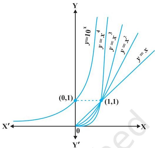 Fig 5.9
Does a function exist that exhibits a growth rate superior to that of any polynomial function? The response is affirmative, and an illustrative instance of such a function is provided below:
$ y = f(x) = 10^{x}. $
We assert that this function $f$ demonstrates a more rapid rate of increase compared to $f_{n}(x) = x^{n}$ for any given positive integer $n$. As an illustration, it can be substantiated that $10^{x}$ outpaces the growth of $f_{100}(x) = x^{100}$. Considering substantial values for $x$, such as $x = 10^{3}$, observe that $f_{100}(x)$ computes to $(10^{3})^{100} = 10^{300}$, whereas $f(10^{3})$ yields $10^{10^{3}} = 10^{1000}$. Evidently, $f(x)$ significantly exceeds $f_{100}(x)$. While a formal demonstration is straightforward for all $x > 10^{3}$, establishing $f(x) > f_{100}(x)$, we shall refrain from presenting such a proof in this context. Analogously, through the selection of sufficiently large $x$ values, one can confirm that $f(x)$ exhibits superior growth to $f_{n}(x)$ for any positive integer $n$.
Definition 3 An exponential function, defined with a positive base $b > 1$, is formally expressed as
$ y = f(x) = b^{x} $
Figure 5.9 illustrates the graph of $y = 10^{x}$. Readers are encouraged to sketch this function for specific base values such as 2, 3, and 4. Key characteristics of exponential functions include:
(1) The domain encompasses all real numbers, denoted as $\mathbf{R}$. (2) The range consists exclusively of positive real numbers. (3) The coordinate $(0, 1)$ invariably lies on the exponential function's graph, reflecting the property that $b^0 = 1$ for any real base $b > 1$. (4) Exponential functions exhibit monotonic increase; specifically, their graphical representation ascends continuously from left to right.
(5) As $x$ tends towards significantly large negative values, the exponential function's output approaches zero. This implies that within the second quadrant, the graph asymptotically approaches the $x$-axis without intersecting it.
When the base is 10, the exponential function is termed the common exponential function. As noted in Appendix A.1.4 of the Class XI curriculum, the series summation
$ 1 + \frac {1}{1 !} + \frac {1}{2 !} + \dots $
converges to a value between 2 and 3, designated by $e$. Employing $e$ as the base yields a profoundly significant exponential function, $y = e^{x}$, which is known as the natural exponential function.
An inquiry into the existence and meaningful interpretation of the inverse of the exponential function naturally leads to the subsequent definition.
Definition 4 Given a real number $b > 1$, the logarithm of $a$ to the base $b$ is defined as $x$ if and only if $b^x = a$. This relationship is symbolically represented as $\log_b a$. Therefore, $\log_b a = x$ is equivalent to $b^x = a$.
To illustrate this concept, consider several explicit instances. The exponential statement $2^3 = 8$ can be equivalently expressed in logarithmic form as $\log_2 8 = 3$. Likewise, $10^4 = 10000$ translates to $\log_{10} 10000 = 4$. Furthermore, the equivalence $625 = 5^4 = 25^2$ implies that $\log_5 625 = 4$ or $\log_{25} 625 = 2$.
From a more advanced perspective, by establishing a base $b > 1$, the logarithm can be conceptualized as a function mapping positive real numbers to the entire set of real numbers. This function, known as the logarithmic function, is formally defined as:
$ \begin{array}{l} \log_ {b}: \mathbf {R} ^ {x} \longrightarrow \mathbf {R} \ x \rightarrow \log_ {b} x = y \quad \text {if} \ b ^ {y} = x \ \end{array} $
Consistent with prior definitions, a base of $b = 10$ signifies common logarithms, whereas a base of $b = e$ indicates natural logarithms. The natural logarithm is frequently symbolized as $\ln$. Within the context of this chapter, the notation $\log x$ will specifically refer to the logarithm function with base $e$, meaning $\ln x$ will be simplified to $\log x$. Figure 5.10 presents graphical representations of the logarithmic function for bases 2, $e$, and 10.
Several crucial characteristics pertaining to the logarithm function, for any base $b > 1$, are enumerated below:
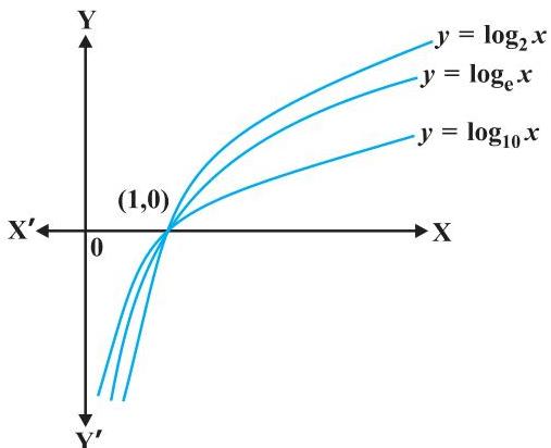 Fig 5.10
(1) The logarithm function is not meaningfully defined for non-positive numbers, which establishes its domain as the set of all positive real numbers ($\mathbf{R}^{+}$).
(2) The codomain of the logarithmic function encompasses all real numbers.
(3) The graphical representation of the logarithmic function invariably includes the coordinate pair $(1, 0)$.
(4) The logarithmic function exhibits monotonic growth; its graph ascends continuously when traversed from left to right.
(5) As $x$ approaches zero from the positive direction, the value of $\log x$ can be arbitrarily small (i.e., approach negative infinity). Graphically, this signifies that the function's curve asymptotically approaches the $y$-axis within the fourth quadrant without ever intersecting it.
(6) Figure 5.11 illustrates the graphs of $y = e^{x}$ and $y = \ln x$. A notable characteristic is their reciprocal relationship, as they appear as reflections of one another across the line $y = x$.
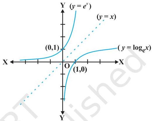 Fig 5.11
Two properties of 'log' functions are proved below:
(1) A fundamental rule for changing the base of logarithms allows expressing $\log_{a}p$ using $\log_b p$. Consider the definitions: $\log_a p = \alpha$, $\log_b p = \beta$, and $\log_b a = \gamma$. These equivalences translate to $a^\alpha = p$, $b^\beta = p$, and $b^\gamma = a$. By substituting the expression for $a$ from the third equation into the first, we derive:
$ (b ^ {\gamma}) ^ {\alpha} = b ^ {\gamma \alpha} = p $
Incorporating this result into the second exponential equivalence yields:
$ b ^ {\beta} = p = b ^ {\gamma \alpha} $
This equality implies that $\beta = \alpha \gamma$, or equivalently, $\alpha = \frac{\beta}{\gamma}$. Consequently, we establish the identity:
$ \log_ {a} p = \frac {\log_ {b} p}{\log_ {b} a} $
(2) A further significant characteristic of the logarithmic function pertains to its interaction with products. Let $\log_b pq = \alpha$, which implies $b^\alpha = pq$. If we define $\log_b p = \beta$ and $\log_b q = \gamma$, then their exponential forms are $b^\beta = p$ and $b^\gamma = q$. Therefore, we can write $b^\alpha = pq = b^\beta b^\gamma = b^{\beta + \gamma}$
This equivalence leads to $\alpha = \beta +\gamma$, meaning:
$ \log_ {b} p q = \log_ {b} p + \log_ {b} q
$
A particularly noteworthy implication arises when $p$ is equal to $q$. Under this condition, the preceding relationship can be restated as:
$ \log_b p^2 = \log_b p + \log_b p = 2 \log p $
A straightforward generalization of this principle (offered as an exercise) is:
$ \log_b p^n = n \log p $
for any positive integer $n$. This holds true for any positive integer $n$, and indeed extends to any real number $n$, though a formal proof for the latter will not be provided here. Following a similar logical progression, the reader is encouraged to confirm the identity:
$ \log_b \frac{x}{y} = \log_b x - \log_b y $
Example 25 Is it true that $x = e^{\log x}$ for all real $x$?
Solution Initially, it is crucial to recognize that the domain of the logarithmic function is restricted to positive real numbers. Consequently, the given assertion is invalid for any non-positive real numbers. Now, consider the expression $y = e^{\log x}$. Assuming $y > 0$, we can apply the logarithm to both sides, yielding $\log y = \log (e^{\log x})$. This simplifies to $\log y = \log x \cdot \log e$, and since $\log e = 1$ (for natural logarithm), we have $\log y = \log x$. This implies that $y = x$. Therefore, the identity $x = e^{\log x}$ holds exclusively for positive real values of $x$.
A remarkable characteristic of the natural exponential function within differential calculus is its invariance under the operation of differentiation. This attribute is formally stated in the subsequent theorem, for which the proof will be omitted.
Theorem 5*
(1) The differentiation of $e^x$ with respect to $x$ results in $e^x$; this is formally stated as $\frac{d}{dx}(e^x) = e^x$.
(2) When $\log x$ is differentiated with respect to $x$, the outcome is $\frac{1}{x}$; expressed mathematically, $\frac{d}{dx} (\log x) = \frac{1}{x}$.
Example 26 Calculate the derivative of the subsequent functions concerning $x$:
(i) $e^{-x}$
(ii) $\sin (\log x), x > 0$
(iii) $\cos^{-1}(e^x)$
(iv) $e^{\cos x}$
Solution
(i) For the function $y = e^{-x}$, applying the chain rule yields:
$ \frac{dy}{dx} = e^{-x} \cdot \frac{d}{dx} (-x) = -e^{-x} $
(ii) Considering $y = \sin (\log x)$, the chain rule dictates that:
$ \frac{dy}{dx} = \cos (\log x) \cdot \frac{d}{dx} (\log x) = \frac{\cos (\log x)}{x} $
(iii) Given $y = \cos^{-1}(e^x)$, the application of the chain rule leads to:
$ \frac{dy}{dx} = \frac{-1}{\sqrt{1 - (e^x)^2}} \cdot \frac{d}{dx} (e^x) = \frac{-e^x}{\sqrt{1 - e^{2x}}} $
(iv) If $y = e^{\cos x}$, employing the chain rule results in:
$ \frac{dy}{dx} = e^{\cos x} \cdot (-\sin x) = -(\sin x) e^{\cos x} $
EXERCISE 5.4
Differentiate the following with respect to $x$:
- $\frac{e^x}{\sin x}$
- $e^{\sin^{-1} x}$
- $e^{x^3}$
- $\sin (\tan^{-1} e^{-x})$
- $\log (\cos e^x)$
- $e^x + e^{x^2} + \ldots + e^{x^3}$
- $\sqrt{e^{\sqrt{x}}}, x > 0$
- $\log (\log x), x > 1$
- $\frac{\cos x}{\log x}, x > 0$
- $\cos (\log x + e^x), x > 0$
5.5. Logarithmic Differentiation
This section introduces the method for differentiating a particular class of functions expressed in the form:
$ y = f(x) = [u(x)]^{v(x)} $
By applying the natural logarithm (to base $e$) to both sides, the expression can be transformed into:
$ \log y = v(x) \log [u(x)] $
Differentiation of this transformed equation with respect to $x$, using the chain rule, yields:
$ \frac{1}{y} \cdot \frac{dy}{dx} = v(x) \cdot \frac{1}{u(x)} \cdot u'(x) + v'(x) \cdot \log [u(x)] $
Consequently, solving for $\frac{dy}{dx}$ gives:
$ \frac{dy}{dx} = y \left[ \frac{v(x)}{u(x)} \cdot u'(x) + v'(x) \cdot \log [u(x)] \right] $
A critical aspect of this technique is the requirement that both $f(x)$ and $u(x)$ maintain positive values, as their logarithms are undefined otherwise. This differentiation procedure is termed logarithmic differentiation and is demonstrated through the subsequent examples:
Example 27 Determine the derivative of $\sqrt{\frac{(x - 3)(x^2 + 4)}{3x^2 + 4x + 5}}$ with respect to $x$.
Solution Assign $y$ to the given function: $y = \sqrt{\frac{(x - 3)(x^2 + 4)}{(3x^2 + 4x + 5)}}$
Applying the logarithm to both sides yields:
$ \log y = \frac {1}{2} \left[ \log (x - 3) + \log (x ^ {2} + 4) - \log (3 x ^ {2} + 4 x + 5) \right] $
Subsequently, differentiating both sides with respect to $x$ results in:
$ \frac {1}{y} \cdot \frac {d y}{d x} = \frac {1}{2} \left[ \frac {1}{(x - 3)} + \frac {2 x}{x ^ {2} + 4} - \frac {6 x + 4}{3 x ^ {2} + 4 x + 5} \right] $
Thus,
$ \begin{array}{l} \frac {d y}{d x} = \frac {y}{2} \left[ \frac {1}{(x - 3)} + \frac {2 x}{x ^ {2} + 4} - \frac {6 x + 4}{3 x ^ {2} + 4 x + 5} \right] \ = \frac {1}{2} \sqrt {\frac {(x - 3) (x ^ {2} + 4)}{3 x ^ {2} + 4 x + 5}} \left[ \frac {1}{(x - 3)} + \frac {2 x}{x ^ {2} + 4} - \frac {6 x + 4}{3 x ^ {2} + 4 x + 5} \right] \ \end{array} $
Example 28 Compute the derivative of $a^x$ concerning $x$, given that $a$ is a positive constant.
Solution Let $y$ be defined as $y = a^{x}$. Consequently:
$ \log y = x \log a $
Differentiating both sides with respect to $x$, we obtain:
$ \frac {1}{y} \frac {d y}{d x} = \log a $
Leading to:
$ \frac {d y}{d x} = y \log a $
Therefore:
$ \frac {d}{d x} \left(a ^ {x}\right) = a ^ {x} \log a $
An alternative approach is as follows:
$ \begin{array}{l} \frac {d}{d x} \left(a ^ {x}\right) = \frac {d}{d x} \left(e ^ {x \log a}\right) = e ^ {x \log a} \frac {d}{d x} (x \log a) \ = e ^ {x \log a} \cdot \log a = a ^ {x} \log a. \ \end{array} $
Example 29 Find the derivative of $x^{\sin x}$ with respect to $x$, for $x > 0$.
Solution Let $y = x^{\sin x}$. Applying the logarithm to both sides yields:
$ \log y = \sin x \log x $
Consequently, differentiating implies:
$ \frac{1}{y} \cdot \frac{dy}{dx} = \sin x \cdot \frac{d}{dx} (\log x) + \log x \cdot \frac{d}{dx} (\sin x) $
or
$ \frac{1}{y} \cdot \frac{dy}{dx} = (\sin x) \cdot \frac{1}{x} + \log x \cos x $
or
$ \frac{dy}{dx} = y \left[ \frac{\sin x}{x} + \cos x \log x \right] $
$ \begin{array}{l} = x^{\sin x} \left[ \frac{\sin x}{x} + \cos x \log x \right] \ = x^{\sin x - 1} \cdot \sin x + x^{\sin x} \cdot \cos x \log x \ \end{array} $
Example 30 Find $\frac{dy}{dx}$, if $y^x + x^y + x^x = a^b$.
Solution We are provided with the equation $y^x + x^y + x^x = a^b$.
By introducing the substitutions $u = y^x$, $v = x^y$, and $w = x^x$, the given equation transforms into $u + v + w = a^b$.
Consequently, differentiating this sum with respect to $x$ yields $\frac{du}{dx} + \frac{dv}{dx} + \frac{dw}{dx} = 0$ (1).
Consider the term $u = y^x$. Applying the natural logarithm to both sides gives:
$ \log u = x \log y $
Differentiating implicitly with respect to $x$ on both sides yields:
$ \begin{array}{l} \frac{1}{u} \cdot \frac{du}{dx} = x \cdot \frac{d}{dx} (\log y) + \log y \cdot \frac{d}{dx} (x) \ = x \cdot \frac{1}{y} \cdot \frac{dy}{dx} + \log y \cdot 1 \ \end{array} $
Thus, the derivative $\frac{du}{dx}$ is expressed as $u \left( \frac{x}{y} \cdot \frac{dy}{dx} + \log y \right)$, which, upon substituting $u = y^x$, becomes $y^x \left[ \frac{x}{y} \cdot \frac{dy}{dx} + \log y \right]$ (2).
Next, we address the term $v = x^y$.
Taking the natural logarithm of both sides, we obtain:
$ \log v = y \log x $
Differentiating implicitly with respect to $x$ yields:
$ \begin{array}{l} \frac{1}{v} \cdot \frac{dv}{dx} = y \cdot \frac{d}{dx} (\log x) + \log x \cdot \frac{dy}{dx} \ = y \cdot \frac{1}{x} + \log x \cdot \frac{dy}{dx} \end{array} $
Consequently,
$ \begin{array}{l} \frac{dv}{dx} = v \left[ \frac{y}{x} + \log x \cdot \frac{dy}{dx} \right] \ = x^y \left[ \frac{y}{x} + \log x \cdot \frac{dy}{dx} \right] \tag{3} \end{array} $
Finally, for the term $w = x^x$.
Taking the natural logarithm on both sides produces:
$ \log w = x \log x. $
Implicit differentiation with respect to $x$ leads to:
$ \begin{array}{l} \frac{1}{w} \cdot \frac{dw}{dx} = x \cdot \frac{d}{dx} (\log x) + \log x \cdot \frac{d}{dx} (x) \ = x \cdot \frac{1}{x} + \log x \cdot 1 \end{array}
$
That is,
$ \begin{array}{l} \frac{dw}{dx} = w (1 + \log x) \ = x^x (1 + \log x) \tag{4} \end{array} $
Substituting the expressions for $\frac{du}{dx}$, $\frac{dv}{dx}$, and $\frac{dw}{dx}$ from (2), (3), and (4) into equation (1), we obtain:
$ \begin{aligned} &y^x \left( \frac{x}{y} \cdot \frac{dy}{dx} + \log y \right) \ &\quad + x^y \left( \frac{y}{x} + \log x \cdot \frac{dy}{dx} \right) \ &\quad + x^x (1 + \log x) = 0 \end{aligned} $
Rearranging the terms to isolate $\frac{dy}{dx}$ gives:
$ \begin{aligned} \left( x \cdot y^{x-1} + x^y \cdot \log x \right) \frac{dy}{dx} &= -x^x (1 + \log x) \ &\quad - y \cdot x^{y-1} \ &\quad - y^x \log y \end{aligned} $
Hence, the final derivative $\frac{dy}{dx}$ is determined as:
$ \frac{dy}{dx} = \frac{ - \left[ y^x \log y + y \cdot x^{y-1} + x^x (1 + \log x) \right] }{ x \cdot y^{x-1} + x^y \log x } $
EXERCISE 5.5
For problems 1 through 11, compute the derivative of the provided functions with respect to $x$.
- $\cos x \cdot \cos 2x \cdot \cos 3x$
- $\sqrt{\frac{(x - 1)(x - 2)}{(x - 3)(x - 4)(x - 5)}}$
- $(\log x)^{\cos x}$
- $x^{x} - 2^{\sin x}$
- $(x + 3)^2 \cdot (x + 4)^3 \cdot (x + 5)^4$
- $\left(x + \frac{1}{x}\right)^x + x^{\left(1 + \frac{1}{x}\right)}$
- $(\log x)^{x} + x^{\log x}$
- $(\sin x)^{x} + \sin^{-1}\sqrt{x}$
- $x^{\sin x} + (\sin x)^{\cos x}$
- $x^{x\cos x} + \frac{x^2 + 1}{x^2 - 1}$
- $(x\cos x)^{x} + (x\sin x)^{\frac{1}{x}}$
For the functions provided in problems 12 through 15, ascertain $\frac{dy}{dx}$.
- $x^{y} + y^{x} = 1$
- $y^{x} = x^{y}$
- $(\cos x)^{y} = (\cos y)^{x}$
- $xy = e^{(x - y)}$
- Determine the derivative of the function $f(x) = (1 + x)(1 + x^2)(1 + x^4)(1 + x^8)$, and subsequently evaluate $f'(1)$.
- Compute the derivative of the expression $(x^{2} - 5x + 8)(x^{3} + 7x + 9)$ using the three methodologies outlined below:
(i) via the application of the product rule (ii) through the expansion of the product into a single polynomial expression (iii) by employing logarithmic differentiation
Do these distinct approaches yield an identical result?
- Given that $u$, $v$, and $w$ are functions of $x$, demonstrate that
$ \frac{d}{dx}(u, v, w) = \frac{du}{dx}vw + u \cdot \frac{dv}{dx} \cdot w + u \cdot v \cdot \frac{dw}{dx} $
utilizing two distinct methods: initially, through the iterative application of the product rule, and subsequently, by employing logarithmic differentiation.
5.6 Derivatives of Functions in Parametric Forms
The relationship between two variables is occasionally neither explicitly defined nor implicitly suggested, but rather established through a mediating third variable that separately links to each of the initial two variables. In such instances, the connection between
the variables is described as being expressed parametrically. This intermediary variable is known as the parameter. Specifically, a relationship between two variables, $x$ and $y$, articulated in the format $x = f(t)$ and $y = g(t)$, is referred to as a parametric form, with $t$ serving as the parameter.
To determine the derivative of a function presented in this configuration, we employ the chain rule:
$ \frac{dy}{dt} = \frac{dy}{dx} \cdot \frac{dx}{dt} $
Alternatively, this can be rearranged to yield:
$ \frac{dy}{dx} = \frac{\frac{dy}{dt}}{\frac{dx}{dt}} \left( \text{whenever } \frac{dx}{dt} \neq 0 \right) $
Consequently, if $y=g(t)$ and $x=f(t)$, the derivative is given by:
$ \begin{aligned} \frac{dy}{dx} &= \frac{g'(t)}{f'(t)} \ &\quad \text{(since } \frac{dy}{dt} = g'(t) \text{ and } \frac{dx}{dt} = f'(t)\text{)} \ &\quad \text{[provided } f'(t) \neq 0\text{]} \end{aligned} $ Example 31 Find $\frac{dy}{dx}$, if $x = a\cos\theta, y = a\sin\theta$.
Solution The given parametric equations are:
$ x = a\cos\theta, \quad y = a\sin\theta $
Differentiating both equations with respect to $\theta$, we obtain:
$ \frac{dx}{d\theta} = -a\sin\theta, \quad \frac{dy}{d\theta} = a\cos\theta $
Thus, the derivative $\frac{dy}{dx}$ is calculated as:
$ \frac{dy}{dx} = \frac{\frac{dy}{d\theta}}{\frac{dx}{d\theta}} = \frac{a\cos\theta}{-a\sin\theta} = -\cot\theta $
Example 32 Find $\frac{dy}{dx}$, if $x = at^2$, $y = 2at$.
Solution The provided parametric equations are $x = at^2$ and $y = 2at$.
Differentiating with respect to $t$:
$ \frac{dx}{dt} = 2at \quad \text{and} \quad \frac{dy}{dt} = 2a $
Consequently, $\frac{dy}{dx}$ is determined by:
$ \frac{dy}{dx} = \frac{\frac{dy}{dt}}{\frac{dx}{dt}} = \frac{2a}{2at} = \frac{1}{t} $
Example 33 Find $\frac{dy}{dx}$, if $x = a(\theta + \sin \theta)$, $y = a(1 - \cos \theta)$.
Solution We are given the equations: $x = a(\theta + \sin \theta)$ and $y = a(1 - \cos \theta)$. Differentiating with respect to $\theta$: $\frac{dx}{d\theta} = a(1 + \cos \theta)$ and $\frac{dy}{d\theta} = a(\sin \theta)$.
Hence, the derivative $\frac{dy}{dx}$ is:
$ \frac{dy}{dx} = \frac{\frac{dy}{d\theta}}{\frac{dx}{d\theta}} = \frac{a\sin\theta}{a(1 + \cos\theta)} = \tan \frac{\theta}{2} $
Note It is pertinent to observe that $\frac{dy}{dx}$ is presented solely in terms of the parameter, without direct reference to the primary variables $x$ and $y$.
Example 34 Find $\frac{dy}{dx}$, if $x^{\frac{2}{3}} + y^{\frac{2}{3}} = a^{\frac{2}{3}}$.
Solution Let us introduce the parametric substitutions $x = a\cos^3\theta$ and $y = a\sin^3\theta$. Substituting these into the given equation:
$ \begin{array}{l} x ^ {\frac {2}{3}} + y ^ {\frac {2}{3}} = (a \cos^ {3} \theta) ^ {\frac {2}{3}} + (a \sin^ {3} \theta) ^ {\frac {2}{3}} \ = a ^ {\frac {2}{3}} \left(\cos^ {2} \theta + \sin^ {2} \theta\right) = a ^ {\frac {2}{3}} \ \end{array} $
This confirms that $x = a\cos^3\theta, y = a\sin^3\theta$ constitute a parametric representation for the equation $x^{\frac{2}{3}} + y^{\frac{2}{3}} = a^{\frac{2}{3}}$.
Now, we differentiate these parametric equations with respect to $\theta$: $\frac{dx}{d\theta} = -3a\cos^2\theta \sin \theta$ and $\frac{dy}{d\theta} = 3a\sin^2\theta \cos \theta$.
Therefore, $\frac{dy}{dx}$ is given by:
$ \frac{dy}{dx} = \frac{\frac{dy}{d\theta}}{\frac{dx}{d\theta}} = \frac{3a\sin^2\theta\cos\theta}{-3a\cos^2\theta\sin\theta} = -\tan \theta = -\sqrt[3]{\frac{y}{x}}
$
EXERCISE 5.6
For Exercises 1 to 10, given $x$ and $y$ are parametrically linked by the provided equations, compute $\frac{dy}{dx}$ without removing the parameter.
- $x = 2at^2, y = at^4$
- $x = a\cos \theta, y = b\cos \theta$
- $x = \sin t, y = \cos 2t$
- $x = 4t, y = \frac{4}{t}$
- $x = \cos \theta - \cos 2\theta, y = \sin \theta - \sin 2\theta$
- $x = a(\theta - \sin \theta), y = a(1 + \cos \theta)$
- $x = \frac{\sin^3 t}{\sqrt{\cos 2t}}, y = \frac{\cos^3 t}{\sqrt{\cos 2t}}$
- $x = a\left(\cos t + \log \tan \frac{t}{2}\right), y = a \sin t$
- $x = a \sec \theta, y = b \tan \theta$
- $x = a(\cos \theta + \theta \sin \theta), y = a(\sin \theta - \theta \cos \theta)$
- If $x = \sqrt{a^{\sin^{-1}t}}, y = \sqrt{a^{\cos^{-1}t}}$, show that $\frac{dy}{dx} = -\frac{y}{x}$
5.7 Second Order Derivative
Start with $y = f(x)$. The first derivative is expressed as:
$ \frac{dy}{dx} = f'(x) \tag{1} $
Should $f'(x)$ possess differentiability, a subsequent differentiation of equation (1) with respect to $x$ is possible. In this operation, the expression on the left-hand side transforms into $\frac{d}{dx}\left(\frac{dy}{dx}\right)$, which is conventionally termed the second-order derivative of $y$ concerning $x$. This is represented by the notation $\frac{d^2y}{dx^2}$. Correspondingly, the second-order derivative of $f(x)$ is indicated by $f''(x)$. Alternative notations include $D^2y$, $y''$, or $y_2$, when $y = f(x)$. It is worth noting that derivatives of orders exceeding two can be conceptualized and defined through an analogous process.
Example 35 Determine $\frac{d^2y}{dx^2}$ for the function $y = x^3 + \tan x$.
Solution The given function is $y = x^3 + \tan x$. The first derivative with respect to $x$ is:
$ \frac{dy}{dx} = 3x^2 + \sec^2 x $
Consequently, the second derivative is obtained by differentiating this expression:
$ \begin{aligned} \frac{d^2y}{dx^2} &= \frac{d}{dx} (3x^2 + \sec^2 x) \ &= 6x + 2\sec x \cdot \sec x \tan x \ &= 6x + 2\sec^2 x \tan x \end{aligned} $
Example 36 Given $y = A \sin x + B \cos x$, demonstrate that $\frac{d^2y}{dx^2} + y = 0$.
Solution We proceed by finding the derivatives:
$ \frac{dy}{dx} = A \cos x - B \sin x $
Subsequently, the second derivative is:
$ \frac{d^2y}{dx^2} = \frac{d}{dx} (A \cos x - B \sin x) = -A \sin x - B \cos x = -y $
Therefore, it follows that:
$ \frac{d^2y}{dx^2} + y = 0 $
Example 37 For the function $y = 3e^{2x} + 2e^{3x}$, establish that $\frac{d^2y}{dx^2} - 5\frac{dy}{dx} + 6y = 0$.
Solution The function provided is $y = 3e^{2x} + 2e^{3x}$. The first derivative is calculated as:
$ \frac{dy}{dx} = 6e^{2x} + 6e^{3x} = 6(e^{2x} + e^{3x}) $
Consequently, the second derivative is found to be:
$ \frac{d^2y}{dx^2} = 12e^{2x} + 18e^{3x} = 6(2e^{2x} + 3e^{3x}) $
Thus, substituting these derivatives and the original function into the expression yields:
$ \begin{aligned} \frac{d^2y}{dx^2} - 5\frac{dy}{dx} + 6y &= 6(2e^{2x} + 3e^{3x}) \ &\quad - 30(e^{2x} + e^{3x}) \ &\quad + 6(3e^{2x} + 2e^{3x}) \ &= 0
\end{aligned} $
Example 38 Given $y = \sin^{-1} x$, demonstrate that $(1 - x^2) \frac{d^2 y}{dx^2} - x \frac{dy}{dx} = 0$.
Solution We begin with $y = \sin^{-1} x$. The first derivative is:
$ \frac{dy}{dx} = \frac{1}{\sqrt{(1 - x^2)}} $
This can be rearranged to:
$ \sqrt{(1 - x^2)} \frac{dy}{dx} = 1 $
Differentiating both sides with respect to $x$ yields:
$ \frac{d}{dx} \left( \sqrt{(1 - x^2)} \cdot \frac{dy}{dx} \right) = 0 $
Applying the product rule, we obtain:
$ \sqrt{(1 - x^2)} \cdot \frac{d^2 y}{dx^2} + \frac{dy}{dx} \cdot \frac{d}{dx} \left( \sqrt{(1 - x^2)} \right) = 0 $
Which simplifies to:
$ \sqrt{(1 - x^2)} \cdot \frac{d^2 y}{dx^2} - \frac{dy}{dx} \cdot \frac{2x}{2\sqrt{1 - x^2}} = 0 $
Consequently,
$ (1 - x^2) \frac{d^2 y}{dx^2} - x \frac{dy}{dx} = 0 $
To demonstrate this relationship, consider the function $y = \sin^{-1} x$. From this, we derive:
$ y_1 = \frac{1}{\sqrt{1 - x^2}}, \text{ i.e., } (1 - x^2) y_1^2 = 1 $
Consequently,
$ (1 - x^2) \cdot 2y_1 y_2 + y_1^2 (0 - 2x) = 0 $
Thus,
$ (1 - x^2) y_2 - x y_1 = 0 $
EXERCISE 5.7
For the functions provided in problems 1 through 10, compute their second-order derivatives.
$x^2 + 3x + 2$
$x^{20}$
$x \cdot \cos x$
$\log x$
$x^3 \log x$
$e^x \sin 5x$
$e^{6x} \cos 3x$
$\tan^{-1} x$
$\log (\log x)$
$\sin (\log x)$
Given $y = 5 \cos x - 3 \sin x$, demonstrate that $\frac{d^2 y}{dx^2} + y = 0$
Given $y = \cos^{-1} x$, determine $\frac{d^2y}{dx^2}$ expressed exclusively in terms of $y$.
Assuming $y = 3 \cos (\log x) + 4 \sin (\log x)$, verify that $x^{2}y_{2} + xy_{1} + y = 0$
Given $y = \mathrm{A}e^{mx} + \mathrm{B}e^{nx}$, establish the relation $\frac{d^2y}{dx^2} - (m + n)\frac{dy}{dx} + mny = 0$
Provided $y = 500e^{7x} + 600e^{-7x}$, verify that $\frac{d^2y}{dx^2} = 49y$
If $e^{y}(x + 1) = 1$, establish the identity $\frac{d^2y}{dx^2} = \left(\frac{dy}{dx}\right)^2$
Provided $y = (\tan^{-1} x)^2$, show that $(x^2 + 1)^2 y_2 + 2x(x^2 + 1) y_1 = 2$
Miscellaneous Examples
Example 39 Differentiate w.r.t. $x$, the following function:
(i) $\sqrt{3x + 2} + \frac{1}{\sqrt{2x^2 + 4}}$
(ii) $\log_7(\log x)$
Solution
(i) Let $y = \sqrt{3x + 2} + \frac{1}{\sqrt{2x^2 + 4}} = (3x + 2)^{\frac{1}{2}} + (2x^2 + 4)^{-\frac{1}{2}}$
It is important to observe that this function's domain encompasses all real numbers $x$ such that $x > -\frac{2}{3}$. Consequently, $ \begin{aligned} \frac{dy}{dx} &= \frac{1}{2} (3x + 2)^{\frac{1}{2} - 1} \cdot \frac{d}{dx} (3x + 2) \ &\quad + \left(-\frac{1}{2}\right) (2x^2 + 4)^{-\frac{1}{2} - 1} \cdot \frac{d}{dx} (2x^2 + 4) \ \ &= \frac{1}{2} (3x + 2)^{-\frac{1}{2}} \cdot 3
- \frac{1}{2} (2x^2 + 4)^{-\frac{3}{2}} \cdot 4x \ \ &= \frac{3}{2\sqrt{3x + 2}}
- \frac{2x}{(2x^2 + 4)^{\frac{3}{2}}} \end{aligned} $
The resulting derivative is valid for all real numbers $x$ satisfying $x > -\frac{2}{3}$.
(ii) Consider $y = \log_7(\log x) = \frac{\log(\log x)}{\log 7}$ (utilizing the change of base formula).
The domain of this function includes all real numbers $x$ where $x > 1$. Hence,
$ \begin{array}{l} \frac{dy}{dx} = \frac{1}{\log 7} \cdot \frac{d}{dx} (\log (\log x)) \ = \frac{1}{\log 7} \cdot \frac{1}{\log x} \cdot \frac{d}{dx} (\log x) \ = \frac{1}{x \log 7 \log x} \end{array} $
Example 40 Differentiate the following w.r.t. $x$.
(i) $\cos^{-1}(\sin x)$ (ii) $\tan^{-1}\left(\frac{\sin x}{1 + \cos x}\right)$ (iii) $\sin^{-1}\left(\frac{2^{x+1}}{1 + 4^x}\right)$
Solution
(i) Let $f(x) = \cos^{-1}(\sin x)$. It can be noted that this function possesses a domain encompassing all real numbers. We can express this function in an alternative form:
$ \begin{array}{l} f(x) = \cos^{-1}(\sin x) \ = \cos^{-1}\left[\cos\left(\frac{\pi}{2} - x\right)\right] \ = \frac{\pi}{2} - x \end{array} $
Therefore, the derivative $f'(x)$ is $-1$.
(ii) Let $f(x) = \tan^{-1}\left(\frac{\sin x}{1 + \cos x}\right)$. This function is defined across all real numbers, with the exclusion of points where $\cos x = -1$, which corresponds to odd multiples of $\pi$. We can transform this function into the following expression:
$ \begin{array}{l} f(x) = \tan^{-1}\left(\frac{\sin x}{1 + \cos x}\right) \ = \tan^{-1}\left[\frac{2 \sin\left(\frac{x}{2}\right) \cos\left(\frac{x}{2}\right)}{2 \cos^2 \frac{x}{2}}\right] \end{array} $
$ = \tan^{-1} \left[ \tan \left(\frac {x}{2}\right) \right] = \frac {x}{2} $
It is important to note that the term $\cos \left(\frac{x}{2}\right)$ could be cancelled from both the numerator and the denominator, given that it does not equal zero. Consequently, $f'(x) = \frac{1}{2}$.
(iii) Let $f(x) = \sin^{-1}\left(\frac{2^{x + 1}}{1 + 4^x}\right)$. Determining the domain of this function requires identifying all values of $x$ for which the condition $-1 \leq \frac{2^{x + 1}}{1 + 4^x} \leq 1$ holds true. As the expression in the inequality's center consistently yields a positive value, our task simplifies to identifying all $x$ satisfying $\frac{2^{x + 1}}{1 + 4^x} \leq 1$, which is equivalent to finding all $x$ where $2^{x + 1} \leq 1 + 4^x$. This inequality can be algebraically manipulated into $2 \leq \frac{1}{2^x} + 2^x$, a statement that holds true for all real $x$. Consequently, the function's domain spans the entire set of real numbers
. By substituting $2^x = \tan \theta$, we can re-express this function as follows:
$ \begin{array}{l} f (x) = \sin^ {- 1} \left[ \frac {2 ^ {x + 1}}{1 + 4 ^ {x}} \right] \ = \sin^ {- 1} \left[ \frac {2 ^ {x} \cdot 2}{1 + \left(2 ^ {x}\right) ^ {2}} \right] \ = \sin^ {- 1} \left[ \frac {2 \tan \theta}{1 + \tan^ {2} \theta} \right] \ = \sin^ {- 1} [ \sin 2 \theta ] \ = 2 \theta = 2 \tan^ {- 1} \left(2 ^ {x}\right) \ \end{array} $
Thus
$ \begin{array}{l} f ^ {\prime} (x) = 2 \cdot \frac {1}{1 + \left(2 ^ {x}\right) ^ {2}} \cdot \frac {d}{d x} \left(2 ^ {x}\right) \ = \frac {2}{1 + 4 ^ {x}} \cdot \left(2 ^ {x}\right) \log 2 \ = \frac {2 ^ {x + 1} \log 2}{1 + 4 ^ {x}} \ \end{array}
$
Example 41
Determine the derivative $f'(x)$ for the function $f(x) = (\sin x)^{\sin x}$, given that $0 < x < \pi$.
Solution Consider the function $y = (\sin x)^{\sin x}$. This function is well-defined when its base, $\sin x$, is positive, a condition met within the specified domain $0 < x < \pi$. To facilitate differentiation, we apply the natural logarithm to both sides, yielding:
$ \log y = \log (\sin x)^{\sin x} = \sin x \log (\sin x) $
Then
$ \begin{aligned} \frac{1}{y} \frac{dy}{dx} &= \frac{d}{dx} \big(\sin x \log (\sin x)\big) \ &= \cos x \log (\sin x)
- \sin x \cdot \frac{1}{\sin x} \cdot \cos x \ &= \cos x \log (\sin x) + \cos x \ &= (1 + \log (\sin x)) \cos x \end{aligned} $
Thus
$ \frac{dy}{dx} = y \left( (1 + \log (\sin x)) \cos x \right) = (1 + \log (\sin x)) (\sin x)^{\sin x} \cos x $
Example 42
Given a positive constant $a$, determine $\frac{dy}{dx}$ when
$ y = a^{t + \frac{1}{t}}, \text{ and } x = \left(t + \frac{1}{t}\right)^a $
Solution It is observed that both $y$ and $x$ are well-defined for all real values of $t$ except $t=0$. The derivatives with respect to $t$ are:
$ \begin{aligned} \frac{dy}{dt} &= \frac{d}{dt} \left(a^{t + \frac{1}{t}}\right) = a^{t + \frac{1}{t}} \cdot \frac{d}{dt} \left(t + \frac{1}{t}\right) \cdot \log a \ &\quad = a^{t + \frac{1}{t}} \left(1 - \frac{1}{t^2}\right) \log a \end{aligned} $
Similarly,
$ \begin{aligned} \frac{dx}{dt} &= a \left[ t + \frac{1}{t} \right]^{a - 1} \cdot \frac{d}{dt} \left(t + \frac{1}{t}\right) \ &= a \left[ t + \frac{1}{t} \right]^{a - 1} \cdot \left(1 - \frac{1}{t^2}\right) \end{aligned} $
The condition for $\frac{dx}{dt}$ to be non-zero is $t \neq \pm 1$. Consequently, under the assumption that $t \neq \pm 1$, we can compute $\frac{dy}{dx}$ as:
$ \frac {d y}{d x} = \frac {\frac {d y}{d t}}{\frac {d x}{d t}} = \frac {a ^ {t + \frac {1}{t}} \left(1 - \frac {1}{t ^ {2}}\right) \log a}{a \left[ t + \frac {1}{t} \right] ^ {a - 1} \cdot \left(1 - \frac {1}{t ^ {2}}\right)} = \frac {a ^ {t + \frac {1}{t}} \log a}{a \left(t + \frac {1}{t}\right) ^ {a - 1}} $
Example 43
Compute the derivative of $\sin^2 x$ with respect to $e^{\cos x}$.
Solution To determine this derivative, let $u(x) = \sin^2 x$ and $v(x) = e^{\cos x}$. Our objective is to calculate $\frac{du}{dv}$, which can be expressed as the quotient $\frac{du / dx}{dv / dx}$. The individual derivatives are found to be:
$ \frac {du}{dx} = 2 \sin x \cos x \text{ and } \frac {dv}{dx} = e ^ {\cos x} (- \sin x) = - (\sin x) e ^ {\cos x} $
Therefore,
$ \frac {du}{dv} = \frac {2 \sin x \cos x}{- \sin x e ^ {\cos x}} = - \frac {2 \cos x}{e ^ {\cos x}} $
Miscellaneous Exercise on Chapter 5
For Exercises 1 through 11, differentiate the provided function with respect to $x$.
$(3x^{2} - 9x + 5)^{9}$
$\sin^3 x + \cos^6 x$
$(5x)^{3\cos 2x}$
$\sin^{-1}(x\sqrt{x}), 0 \leq x \leq 1$
$\frac{\cos^{-1}\frac{x}{2}}{\sqrt{2x + 7}}, -2 < x < 2$
$\cot^{-1}\left[\frac{\sqrt{1 + \sin x} + \sqrt{1 - \sin x}}{\sqrt{1 + \sin x} - \sqrt{1 - \sin x}}\right], 0 < x < \frac{\pi}{2}$
$(\log x)^{\log x}, x > 1$
$\cos (a\cos x + b\sin x)$, where $a$ and $b$ are constants.
$(\sin x - \cos x)^{(\sin x - \cos x)}, \frac{\pi}{4} < x < \frac{3\pi}{4}$
$x^{x} + x^{a} + a^{x} + a^{a}$, given a fixed $a > 0$ and $x > 0$.
$x^{x^2 - 3} + (x - 3)^{x^2}$, applicable for
$x > 3$. 12. Determine $\frac{dy}{dx}$ when $y = 12(1 - \cos t)$ and $x = 10(t - \sin t)$, for $-\frac{\pi}{2} < t < \frac{\pi}{2}$. 13. Determine $\frac{dy}{dx}$ given $y = \sin^{-1}x + \sin^{-1}\sqrt{1 - x^2}$, for $0 < x < 1$. 14. Given the equation $x\sqrt{1 + y} + y\sqrt{1 + x} = 0$, valid for $-1 < x < 1$, establish that
$ \frac{dy}{dx} = -\frac{1}{(1 + x)^2} $
- Assuming $(x - a)^2 + (y - b)^2 = c^2$, where $c > 0$ is a constant, demonstrate that
$ \left[1 + \left(\frac{dy}{dx}\right)^2\right]^{\frac{3}{2}} $
remains constant, irrespective of the values of $a$ and $b$.
Provided that $\cos y = x \cos (a + y)$ and $\cos a \neq \pm 1$, establish the derivative $\frac{dy}{dx} = \frac{\cos^2(a + y)}{\sin a}$.
Given $x = a (\cos t + t \sin t)$ and $y = a (\sin t - t \cos t)$, compute $\frac{d^2y}{dx^2}$.
For the function $f(x) = |x|^3$, prove that $f''(x)$ is defined for all real numbers $x$, and subsequently determine its expression.
By employing the identity $\sin (A + B) = \sin A \cos B + \cos A \sin B$ and the principles of differentiation, derive the sum formula for the cosine function.
Is it possible for a function to exhibit continuity across its entire domain while failing to be differentiable at precisely two distinct points? Provide a reasoned justification for your conclusion.
Given $y = \begin{vmatrix} f(x) & g(x) & h(x) \ l & m & n \ a & b & c \end{vmatrix}$, establish the derivative $\frac{dy}{dx} = \begin{vmatrix} f'(x) & g'(x) & h'(x) \ l & m & n \ a & b & c \end{vmatrix}$.
For the function $y = e^{a\cos^{-1}x}$, defined for $-1 \leq x \leq 1$, demonstrate that the following differential equation holds: $(1 - x^2)\frac{d^2y}{dx^2} - x\frac{dy}{dx} - a^2y = 0$.
Summary
A real-valued function is defined as continuous at a specific point within its domain if the function's limit at that point is equivalent to its actual value at that point. A function achieves overall continuity if this condition holds true across its entire domain.
The collection of continuous functions is closed under basic arithmetic operations. Specifically, if $f$ and $g$ represent continuous functions, then the following operations also yield continuous functions:
$ (f \pm g) (x) = f (x) \pm g (x) \text{ is continuous}. $
$ (f \cdot g) (x) = f (x) \cdot g (x) \text{ is continuous}. $
$ \left(\frac {f}{g}\right) (x) = \frac {f (x)}{g (x)} \quad \text{(wherever } g (x) \neq 0\text{ ) is continuous.} $
Any function that is differentiable inherently possesses continuity; however, the reverse assertion is not universally valid.
The Chain Rule provides a methodology for computing the derivative of composite functions. If $f$ is expressed as the composition $\nu \circ u$, with $t = u(x)$, and provided that both $\frac{dt}{dx}$ and $\frac{dv}{dt}$ exist, then the derivative of $f$ with respect to $x$ is given by:
$ \frac {df}{dx} = \frac {dv}{dt} \cdot \frac {dt}{dx} $
Presented below are several fundamental derivatives, valid within their respective domains:
$ \frac {d}{dx} (\sin^ {- 1} x) = \frac {1}{\sqrt {1 - x ^ {2}}} \quad \frac {d}{dx} (\cos^ {- 1} x) = - \frac {1}{\sqrt {1 - x ^ {2}}} $
$ \frac {d}{dx} (\tan^ {- 1} x) = \frac {1}{1 + x ^ {2}} $
$ \frac {d}{dx} \left(e ^ {x}\right) = e ^ {x} \quad \frac {d}{dx} (\log x) = \frac {1}{x} $
Logarithmic differentiation stands as an effective approach for determining the derivative of functions structured as $f(x) = [u(x)]^{v(x)}$. For this technique to be applicable and meaningful, both $f(x)$ and $u(x)$ must maintain positive values.