Chapter 9
DIFFERENTIAL EQUATIONS
He who seeks for methods without having a definite problem in mind seeks for the most part in vain. – D. HILBERT
9.1 Introduction
In previous academic contexts, specifically in Class XI and Chapter 5 of this textbook, the process of differentiating a function $f$ with respect to an independent variable was explored, entailing the determination of $f'(x)$ for any $x$ within the function's defined domain. Subsequently, within the discussion of Integral Calculus, the inverse problem was addressed: identifying a function $f$ given its derivative $g$. This latter task can be equivalently articulated as follows:
Given a specific function $g$, the objective is to ascertain a function $f$ such that its derivative corresponds to $g$, expressed mathematically as:
$ \frac{dy}{dx} = g(x), \text{ where } y = f(x) \tag{1} $
An expression structured like equation (1) is identified as a differential equation. A more precise and formal definition will be presented subsequently.
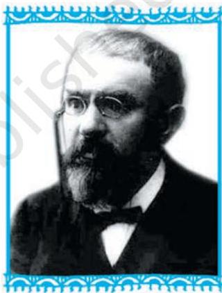 Henri Poincare (1854-1912)
Such equations manifest across a diverse array of disciplines, encompassing fields such as Physics, Chemistry, Biology, Anthropology, Geology, and Economics, among others. Consequently, a comprehensive exploration of differential equations has attained paramount significance within contemporary scientific inquiry.
Within the confines of this chapter, the curriculum will encompass fundamental principles pertaining to differential equations, the distinctions between general and particular solutions, techniques for the formulation of differential equations, various methodologies for solving first-order, first-degree differential equations, and an examination of their practical applications across diverse domains.
9.2 Basic Concepts
Equations of the following form are familiar to us:
$ x^2 - 3x + 3 = 0 \tag{1} $
$ \sin x + \cos x = 0 \tag{2} $
$ x + y = 7 \tag{3}
$
Now, let us examine the equation:
$ x \frac {d y}{d x} + y = 0 \tag {4} $
A key distinction is observed: equations (1), (2), and (3) exclusively feature independent and/or dependent variables, whereas equation (4) includes both variables and the derivative of the dependent variable $y$ with respect to the independent variable $x$. An equation structured in this manner is defined as a differential equation.
More broadly, any equation that incorporates a derivative or multiple derivatives of a dependent variable concerning one or more independent variables is classified as a differential equation.
When a differential equation contains derivatives of the dependent variable solely with respect to a single independent variable, it is referred to as an ordinary differential equation (ODE). For example,
$ \begin{aligned} 2 \frac{d^2 y}{dx^2} + \left(\frac{dy}{dx}\right)^3 = 0, \quad \text{an ordinary differential equation} \tag{5} \end{aligned} $
Naturally, certain differential equations incorporate derivatives with respect to multiple independent variables; these are known as partial differential equations. Nevertheless, our current focus will be exclusively on ordinary differential equations. Henceforth, the designation 'differential equation' will implicitly refer to an 'ordinary differential equation'.
Note
For derivatives, we will predominantly employ the subsequent notations:
$\frac{dy}{dx} = y', \frac{d^2y}{dx^2} = y'', \frac{d^3y}{dx^3} = y'''$
Employing numerous prime symbols for higher-order derivatives becomes impractical. Consequently, we adopt the notation $y_{n}$ to represent the nth-order derivative $\frac{d^n y}{dx^n}$ .
9.2.1. Order of a differential equation
The order attributed to a differential equation corresponds to the highest derivative of the dependent variable concerning the independent variable that appears within that equation.
Consider the following differential equations:
$ \frac {d y}{d x} = e ^ {x} \tag {6} $
$
\frac {d ^ {2} y}{d x ^ {2}} + y = 0 \tag {7} $
$ \left(\frac {d ^ {3} y}{d x ^ {3}}\right) + x ^ {2} \left(\frac {d ^ {2} y}{d x ^ {2}}\right) ^ {3} = 0 \tag {8} $
Equations (6), (7), and (8) feature highest derivatives of the first, second, and third orders, respectively. Consequently, their respective orders are 1, 2, and 3.
9.2.2 Degree of a differential equation
To ascertain the degree of a differential equation, it is crucial that the equation can be expressed as a polynomial in its derivatives, such as $y'$, $y''$, $y'''$, and so forth. Let us examine the subsequent differential equations:
$ \frac {d ^ {3} y}{d x ^ {3}} + 2 \left(\frac {d ^ {2} y}{d x ^ {2}}\right) ^ {2} - \frac {d y}{d x} + y = 0 \tag {9} $
$ \left(\frac {d y}{d x}\right) ^ {2} + \left(\frac {d y}{d x}\right) - \sin^{2} y = 0 \tag {10} $
$ \frac {d y}{d x} + \sin \left(\frac {d y}{d x}\right) = 0 \tag {11} $
It can be observed that equation (9) represents a polynomial expression with respect to $y^{\prime \prime \prime}$, $y^{\prime \prime}$, and $y^\prime$. Similarly, equation (10) constitutes a polynomial in $y^\prime$ (though not in $y$ itself). For such differential equations, the degree is ascertainable. However, equation (11) does not conform to the definition of a polynomial equation in $y^\prime$, and consequently, its degree cannot be determined.
When a differential equation is expressible as a polynomial in its derivatives, its degree is defined as the maximum positive integer exponent of the highest-order derivative present within the equation.
Consistent with the aforementioned definition, it can be noted that differential equations (6), (7), (8), and (9) each possess a degree of one. Equation (10) is of degree two, whereas the degree of differential equation (11) remains undefined.
Note Order and degree (if defined) of a differential equation are always positive integers.
Example 1 Find the order and degree, if defined, of each of the following differential equations:
(i) $\frac{dy}{dx} - \cos x = 0$
(ii) $xy\frac{d^2y}{dx^2} + x\left(\frac{dy}{dx}\right)^2 - y\frac{dy}{dx} = 0$
(iii) $y^{\prime \prime \prime} + y^{2} + e^{y^{\prime}} = 0$
Solution
(i) Within the differential equation, the derivative of the highest order is $\frac{dy}{dx}$, which establishes its order as one. Given that this equation can be expressed as a polynomial in $y'$, and the maximum exponent applied to $\frac{dy}{dx}$ is one, its degree is consequently one.
(ii) The differential equation under consideration contains $\frac{d^2y}{dx^2}$ as its highest order derivative, thus assigning it an order of two. As the equation represents a polynomial in terms of both $\frac{d^2y}{dx^2}$ and $\frac{dy}{dx}$, and the highest power associated with $\frac{d^2y}{dx^2}$ is one, its degree is determined to be one.
(iii) In this differential equation, the highest order derivative found is $y^{\prime \prime \prime}$, which means its order is three. Since the presented differential equation does not conform to a polynomial structure concerning its derivatives, its degree cannot be established.
EXERCISE 9.1
For the differential equations presented in Exercises 1 through 10, ascertain their respective order and, if applicable, their degree.
$\frac{d^4y}{dx^4} +\sin (y^{\prime \prime \prime}) = 0$
$y^{\prime} + 5y = 0$
$\left(\frac{ds}{dt}\right)^4 + 3s\frac{d^2s}{dt^2} = 0$
$\left(\frac{d^2y}{dx^2}\right)^2 +\cos \left(\frac{dy}{dx}\right) = 0$
$\frac{d^2y}{dx^2} = \cos 3x + \sin 3x$
$(y^{\prime \prime \prime})^2 + (y^{\prime \prime})^3 + (y^{\prime})^4 + y^5 = 0$
$y^{\prime \prime \prime} + 2y^{\prime \prime} + y^{\prime} = 0$
$y^{\prime} + y = e^{x}$
$y'' + (y')^2 + 2y = 0$
$y'' + 2y' + \sin y = 0$
The degree of the differential equation
$ \left(\frac {d ^ {2} y}{d x ^ {2}}\right) ^ {3} + \left(\frac {d y}{d x}\right) ^ {2} + \sin \left(\frac {d y}{d x}\right) + 1 = 0 \text{ is} $
(A) 3
(B) 2
(C) 1
(D) not defined
- The order of the differential equation
$ 2 x ^ {2} \frac {d ^ {2} y}{d x ^ {2}} - 3 \frac {d y}{d x} + y = 0 \text{ is} $
(A) 2
(B) 1
(C) 0
(D) not defined
9.3. General and Particular Solutions of a Differential Equation
In previous academic contexts, we encountered and resolved equations such as:
$ x ^ {2} + 1 = 0 \tag {1} $
$ \sin^ {2} x - \cos x = 0 \tag {2} $
The solutions to equations (1) and (2) are numerical values, either real or complex, which satisfy the given equation. This means that upon substituting such a number for the independent variable $x$ in the equation, the left-hand side (L.H.S.) equates to the right-hand side (R.H.S.). $ \begin{aligned} \text{Now consider the differential equation} \ \frac{d^2 y}{dx^2} + y = 0 \tag{3} \end{aligned} $
In contrast to the preceding two equations, the solution for this differential equation is a function, denoted $\phi$, that fulfills its conditions. Specifically, when the function $\phi$ replaces the dependent variable $y$ in the specified differential equation, the L.H.S. becomes equal to the R.H.S..
The graphical representation of $y = \phi(x)$ is referred to as the solution curve (or integral curve) of the given differential equation. Let's examine the function defined as:
$ y = \phi (x) = a \sin (x + b), \tag {4} $
where $a, b \in \mathbf{R}$. If this function and its derivatives are substituted into equation (3), the L.H.S. equals the R.H.S.. Consequently, it constitutes a valid solution to the differential equation (3).
Suppose specific values are assigned to $a$ and $b$, for instance, $a = 2$ and $b = \frac{\pi}{4}$. This yields a specific function:
$ \text{function} \quad y = \phi_ {1} (x) = 2 \sin \left(x + \frac {\pi}{4}\right) \tag {5} $
When this function and its derivative are subsequently substituted into equation (3), the L.H.S. once again equals the R.H.S.. Therefore, $\phi_{1}$ also represents a solution to equation (3).
The function $\phi$ incorporates two arbitrary constants (parameters), $a$ and $b$, and is thus termed the general solution of the given differential equation. Conversely, the function $\phi_1$ contains no arbitrary constants, but rather specific numerical assignments for the parameters $a$ and $b$, and is consequently referred to as a particular solution of the differential equation.
A solution that includes arbitrary constants is designated as the general solution (or primitive) of the differential equation.
A solution devoid of arbitrary constants, meaning one derived from the general solution by assigning specific values to these arbitrary constants, is known as a particular solution of the differential equation.
Example 2 Verify that the function $y = e^{-3x}$ is a solution of the differential equation
$ \frac{d^2 y}{dx^2} + \frac{dy}{dx} - 6y = 0 $
Solution The given function is $y = e^{-3x}$. Differentiating both sides of this expression with respect to $x$ yields:
$ \frac{dy}{dx} = -3e^{-3x} \tag{1} $
Next, differentiating (1) with respect to $x$ provides:
$ \frac{d^2 y}{dx^2} = 9e^{-3x} $
Substituting the derived values of $\frac{d^2 y}{dx^2}$, $\frac{dy}{dx}$, and $y$ into the provided differential equation, we obtain: $ \begin{aligned} \text{L.H.S.} &= 9e^{-3x} - 3e^{-3x} - 6e^{-3x} \ &= 9e^{-3x} - 9e^{-3x} \ &= 0 \ &= \text{R.H.S.} \end{aligned} $
Hence, the specified function indeed serves as a solution to the given differential equation.
Example 3 Verify that the function $y = a\cos x + b\sin x$, where, $a, b \in \mathbf{R}$ is a solution of the differential equation $\frac{d^2 y}{dx^2} + y = 0$
Solution Consider the function defined as:
$ y = a\cos x + b\sin x \tag{1} $
Upon differentiating both sides of expression (1) with respect to the variable $x$, consecutively, the following derivatives are obtained:
$ \frac{dy}{dx} = -a\sin x + b\cos x $
$ \frac{d^2 y}{dx^2} = -a\cos x - b\sin x $
By substituting the expressions for $\frac{d^2y}{dx^2}$ and $y$ into the specified differential equation, the following result is derived:
$ \begin{aligned} \text{L.H.S.} &= (-a\cos x - b\sin x) + (a\cos x + b\sin x) \ &= 0 \ &= \text{R.H.S.} \end{aligned} $
Consequently, the provided function is confirmed to be a valid solution to the given differential equation.
EXERCISE 9.2
For each of the problems numbered 1 through 10, confirm that the provided function (whether explicitly or implicitly defined) satisfies its corresponding differential equation:
$y = e^{x} + 1$ : $y'' - y' = 0$
$y = x^{2} + 2x + C$ : $y' - 2x - 2 = 0$
$y = \cos x + C$ : $y' + \sin x = 0$
$y = \sqrt{1 + x^2}$ : $y' = \frac{xy}{1 + x^2}$
$y = Ax$ : $xy' = y$ ( $x \neq 0$ )
$y = x\sin x$ : $xy' = y + x\sqrt{x^2 - y^2}$ ( $x \neq 0$ and $x > y$ or $x < -y$ )
$xy = \log y + C$ : $y' = \frac{y^2}{1 - xy}$ ( $xy \neq 1$ )
$y - \cos y = x$ : $(y\sin y + \cos y + x)y' = y$
$x + y = \tan^{-1}y$ : $y^{2}y^{\prime} + y^{2} + 1 = 0$
$y = \sqrt{a^2 - x^2} x \in (-a, a)$ : $x + y \frac{dy}{dx} = 0$ ( $y \neq 0$ )
Determine the count of arbitrary constants present in the general solution of a fourth-order differential equation:
(A) 0
(B) 2
(C) 3
(D) 4
- Identify the number of arbitrary constants found in the particular solution of a third-order differential equation:
(A) 3
(B) 2
(C) 1
(D) 0
9.4. Methods of Solving First Order, First Degree Differential Equations
Within this segment, we will delve into three distinct approaches for resolving first-order, first-degree differential equations.
9.4.1 Differential equations with variables separable
A differential equation of the first order and first degree takes the general form:
$ \frac{dy}{dx} = F(x, y) \tag{1} $
Should the function $F(x, y)$ be representable as the product of two functions, $g(x)$ and $h(y)$, where $g(x)$ depends solely on $x$ and $h(y)$ depends solely on $y$, then the differential equation (1) is classified as a variable separable type. In such an instance, differential equation (1) assumes the configuration:
$ \frac{dy}{dx} = h(y) \cdot g(x) \tag{2} $
Provided that $h(y) \neq 0$, the process of separating variables allows equation (2) to be re-expressed as:
$ \frac{1}{h(y)} dy = g(x) dx \tag{3} $
Upon integrating both members of equation (3), one obtains:
$ \int \frac{1}{h(y)} dy = \int g(x) dx \tag{4} $
Consequently, expression (4) yields the solutions for the specified differential equation, presented in the format:
$ H(y) = G(x) + C $
In this context, $H(y)$ and $G(x)$ denote the antiderivatives of $\frac{1}{h(y)}$ and $g(x)$, respectively, with $C$ representing the arbitrary constant of integration.
Example 4 Find the general solution of the differential equation $\frac{dy}{dx} = \frac{x + 1}{2 - y}$, ($y \neq 2$)
Solution We have
$ \frac{dy}{dx} = \frac{x + 1}{2 - y} \tag{1} $
By isolating the variables in equation (1), we arrive at:
$ (2 - y) dy = (x + 1) dx \tag{2} $
The integration of both sides of equation (2) yields:
$ \int (2 - y) dy = \int (x + 1) dx $
or
$ 2y - \frac{y^2}{2} = \frac{x^2}{2} + x + C_1 $
or
$ x^2 + y^2 + 2x - 4y + 2C_1 = 0 $
or
$ x^2 + y^2 + 2x - 4y + C = 0, \text{ where } C = 2C_1 $
This expression represents the general solution for equation (1).
Example 5 Find the general solution of the differential equation $\frac{dy}{dx} = \frac{1 + y^2}{1 + x^2}$ .
Solution Given that $1 + y^2 \neq 0$, the variables can be separated, allowing the initial differential equation to be expressed as:
$ \frac {d y}{1 + y ^ {2}} = \frac {d x}{1 + x ^ {2}} \tag {1} $
Upon integrating both members of equation (1), we obtain:
$ \int \frac {d y}{1 + y ^ {2}} = \int \frac {d x}{1 + x ^ {2}} $
or $ \tan^{-1}y = \tan^{-1}x + C $
This constitutes the general solution for equation (1).
Example 6 Find the particular solution of the differential equation $\frac{dy}{dx} = -4xy^2$ given that $y = 1$, when $x = 0$.
Solution Assuming $y \neq 0$, the provided differential equation may be reformulated as:
$ \frac {d y}{y ^ {2}} = - 4 x d x \tag {1} $
The integration of both sides of equation (1) yields:
$ \int \frac {d y}{y ^ {2}} = - 4 \int x d x $
or $ -\frac{1}{y} = -2x^{2} + C $
or $ y = \frac{1}{2x^2 - C} \tag{2} $
By substituting $y = 1$ and $x = 0$ into equation (2), one determines that $C = -1$.
Subsequently, by re-inserting the determined value of $C$ into equation (2), the particular solution for the initial differential equation is obtained as $y = \frac{1}{2x^2 + 1}$.
Example 7 Find the equation of the curve passing through the point $(1,1)$ whose differential equation is $x dy = (2x^2 + 1) dx$ ($x \neq 0$).
Example 8 Determine the equation of a curve that intersects the point $(-2, 3)$, considering that the gradient of the tangent to this curve at any arbitrary point $(x, y)$ is expressed as $\frac{2x}{y^2}$.
Solution It is established that the slope of a curve's tangent is represented by the derivative $\frac{dy}{dx}$.
Thus,
$ \frac{dy}{dx} = \frac{2x}{y^2} \tag{1} $
By employing the method of separation of variables, equation (1) can be reformulated as
$ y^2 dy = 2x dx \tag{2} $
Upon integrating both sides of equation (2), we arrive at
$ \int y^2 dy = \int 2x dx $
or
$ \frac{y^3}{3} = x^2 + C \tag{3} $
- Leibniz's notation $\frac{dy}{dx}$ offers remarkable flexibility and utility in numerous computational processes and formal transformations, enabling the treatment of the symbols $dy$ and $dx$ akin to ordinary numerical quantities. This approach, treating $dx$ and $dy$ as distinct elements, facilitates the derivation of more concise expressions in a variety of calculations.
For reference, consult: Introduction to Calculus and Analysis, volume I, page 172, By Richard Courant, Fritz John, Springer-Verlag New York.
By substituting the coordinates $x = -2$ and $y = 3$ into equation (3), we determine the constant $C$ to be 5.
Inserting this value of $C$ into equation (3) yields the equation of the desired curve as
$ \frac {y ^ {3}}{3} = x ^ {2} + 5 \quad \text{or} \quad y = (3 x ^ {2} + 15) ^ {\frac {1}{3}} $
Example 9 Consider a banking scenario where the principal continuously grows at an annual rate of $5%$. The question is to determine the number of years it will take for an initial amount of Rs 1000 to double.
Solution Designate $\mathrm{P}$ as the principal at an arbitrary time $t$. As per the problem statement,
$ \frac {dp}{dt} = \left(\frac {5}{100}\right) \times \mathrm{P} $
or
$ \frac {dp}{dt} = \frac {\mathrm{P}}{20} \tag {1} $
By applying variable separation to equation (1), we obtain
$ \frac {dp}{\mathrm{P}} = \frac {dt}{20} \tag {2} $
Upon integrating both sides of equation (2), we find
$ \log \mathrm{P} = \frac {t}{20} + \mathrm{C}_1 $
or
$ \mathrm{P} = e ^ {\frac {t}{20}} \cdot e ^ {\mathrm{C}_1} $
or
$ \mathrm{P} = \mathrm{C} e ^ {\frac {t}{20}} \quad (\text{where} \ e ^ {\mathrm{C}_1} = \mathrm{C}) \tag {3} $
Given the initial conditions,
$ \mathrm{P} = 1000, \quad \text{when } t = 0 $
By substituting the initial values of $\mathrm{P}$ and $t$ into equation (3), we find $C = 1000$. Consequently, equation (3) is refined to
$ \mathrm{P} = 1000 e ^ {\frac {t}{20}} $
Let $t$ denote the duration in years necessary for the principal to double. In that case,
$ 2000 = 1000 e ^ {\frac {t}{20}} \Rightarrow t = 20 \log_ {e} 2 $
EXERCISE 9.3
Obtain the general solution for every differential equation listed in Exercises 1 to 10:
$\frac{dy}{dx} = \frac{1 - \cos x}{1 + \cos x}$
$\frac{dy}{dx} = \sqrt{4 - y^2} \ (-2 < y < 2)$
$\frac{dy}{dx} + y = 1 (y \neq 1)$
$\sec^2 x \tan y , dx + \sec^2 y \tan x , dy = 0$
$(e^{x} + e^{-x}) , dy - (e^{x} - e^{-x}) , dx = 0$
$\frac{dy}{dx} = (1 + x^2)(1 + y^2)$
$y \log y , dx - x , dy = 0$
$x^{5} \frac{dy}{dx} = -y^{5}$
$\frac{dy}{dx} = \sin^{-1} x$
$e^{x} \tan y , dx + (1 - e^{x}) \sec^{2} y , dy = 0$
For each differential equation in Exercises 11 to 14, determine the specific solution that fulfills the provided initial condition:
$(x^{3} + x^{2} + x + 1)\frac{dy}{dx} = 2x^{2} + x; y = 1$ when $x = 0$
$x(x^{2} - 1)\frac{dy}{dx} = 1; y = 0$ when $x = 2$
$\cos \left(\frac{dy}{dx}\right) = a \quad (a \in \mathbf{R}); y = 1$ when $x = 0$
$\frac{dy}{dx} = y \tan x; y = 1$ when $x = 0$
Determine the algebraic expression for a curve that traverses the origin $(0, 0)$ and whose derivative is defined by the differential equation $y' = e^x \sin x$.
Given the differential equation $xy \frac{dy}{dx} = (x + 2)(y + 2)$, identify the specific solution curve that intersects the point $(1, -1)$.
Determine the equation of a curve that includes the point $(0, -2)$, given that at any point $(x, y)$ on the curve, the product of the tangent's slope and the $y$-coordinate equals the $x$-coordinate.
For an arbitrary point $(x, y)$ on a curve, the gradient of the tangent line is twice the gradient of the line segment connecting the point of tangency to the fixed point $(-4, -3)$. Ascertain the curve's equation, knowing that it passes through $(-2, 1)$.
A spherical balloon is being inflated such that its volume increases at a constant rate. If its initial radius is 3 units, and after 3 seconds the radius measures 6 units, calculate the balloon's radius as a function of time $t$ in seconds.
A bank account's principal amount grows continuously at an annual rate of $r%$. Determine the percentage value of $r$ if an initial deposit of Rs 100 doubles its value over a period of 10 years (utilize $\log_e 2 = 0.6931$).
The principal in a bank account experiences continuous growth at an annual rate of $5%$. If Rs 1000 is initially deposited, compute the total value of the investment after 10 years (given $e^{0.5} = 1.648$).
Within a biological culture, the initial bacterial population is 100,000. This population escalates by $10%$ over a 2-hour interval. Assuming the bacterial growth rate is directly proportional to the current population size, ascertain the time required, in hours, for the count to attain 200,000.
The overarching solution to the differential equation $\frac{dy}{dx} = e^{x + y}$ is given by:
(A) $e^{x} + e^{-y} = C$
(B) $e^x + e^y = C$
(C) $e^{-x} + e^{y} = C$
(D) $e^{-x} + e^{-y} = C$
9.4.2 Homogeneous differential equations
Let us examine the following functions involving variables $x$ and $y$:
$ F_1(x, y) = y^2 + 2xy, $
$ F_2(x, y) = 2x - 3y, $
$ F_3(x, y) = \cos\left(\frac{y}{x}\right), $
$ F_4(x, y) = \sin x + \cos y $
When the variables $x$ and $y$ are replaced by $\lambda x$ and $\lambda y$, respectively, for any non-zero constant $\lambda$, the results for these functions are:
$ F_1(\lambda x, \lambda y) = \lambda^2 (y^2 + 2xy) = \lambda^2 F_1(x, y) $
$ F_2(\lambda x, \lambda y) = \lambda (2x - 3y) = \lambda F_2(x, y) $
$ F_3(\lambda x, \lambda y) = \cos\left(\frac{\lambda y}{\lambda x}\right) = \cos\left(\frac{y}{x}\right) = \lambda^0 F_3(x, y) $
$ F_4(\lambda x, \lambda y) = \sin \lambda x + \cos \lambda y \neq \lambda^n F_4(x, y), \text{ for any } n \in \mathbb{N} $
From these examples, it is evident that functions $F_1$, $F_2$, and $F_3$ satisfy the condition $F(\lambda x, \lambda y) = \lambda^n F(x, y)$, whereas $F_4$ does not conform to this pattern. This distinction leads to the formal definition:
A function $F(x, y)$ is defined as a homogeneous function of degree $n$ if $ F(\lambda x, \lambda y) = \lambda^n F(x, y) \text{ for any nonzero constant } \lambda. $
Based on this definition, $F_1$, $F_2$, and $F_3$ are homogeneous functions of degree 2, 1, and 0, respectively, while $F_4$ is not a homogeneous function.
An alternative structural characteristic of these functions can also be observed:
$ \mathrm{F}_1(x, y) = x^2 \left(\frac{y^2}{x^2} + \frac{2y}{x}\right) = x^2 h_1 \left(\frac{y}{x}\right) $
or
$ \mathrm{F}_1(x, y) = y^2 \left(1 + \frac{2x}{y}\right) = y^2 h_2 \left(\frac{x}{y}\right) $
$ \mathrm{F}_2(x, y) = x^1 \left(2 - \frac{3y}{x}\right) = x^1 h_3 \left(\frac{y}{x}\right) $
or
$ \mathrm{F}_2(x, y) = y^1 \left(2\frac{x}{y} - 3\right) = y^1 h_4 \left(\frac{x}{y}\right) $
$ \mathrm{F}_3(x, y) = x^0 \cos \left(\frac{y}{x}\right) = x^0 h_5 \left(\frac{y}{x}\right) $
$ \mathrm{F}_4(x, y) \neq x^n h_6 \left(\frac{y}{x}\right), \text{ for any } n \in \mathbf{N} $
or
$ \mathrm{F}_4(x, y) \neq y^n h_7 \left(\frac{x}{y}\right), \text{ for any } n \in \mathbf{N} $
Consequently, a function $\mathrm{F}(x,y)$ is identified as a homogeneous function of degree $n$ if it can be expressed in the form:
$ \mathrm{F}(x, y) = x^n g \left(\frac{y}{x}\right) \quad \text{or} \quad y^n h \left(\frac{x}{y}\right) $
A differential equation expressed as $\frac{dy}{dx} = \mathrm{F}(x, y)$ is termed homogeneous if the function $\mathrm{F}(x, y)$ itself is a homogeneous function of degree zero.
To obtain solutions for a homogeneous differential equation structured as:
$ \frac{dy}{dx} = \mathrm{F}(x, y) = g \left(\frac{y}{x}\right) \tag{1} $
we introduce the substitution $ y = v \cdot x \tag{2} $
Differentiating equation (2) with respect to $x$ yields:
$ \frac{dy}{dx} = v + x \frac{dv}{dx} \tag{3} $
By substituting the expression for $\frac{dy}{dx}$ from equation (3) into equation (1), we arrive at:
$ v + x \frac{dv}{dx} = g(v) $
which can be rearranged to:
$ x \frac{dv}{dx} = g(v) - v \tag{4} $
Separating the variables in equation (4) results in:
$ \frac{dv}{g(v) - v} = \frac{dx}{x} \tag{5} $
Upon integrating both members of equation (5), one obtains:
$ \int \frac{dv}{g(v) - v} = \int \frac{1}{x} dx + C \tag{6} $
The general solution (or primitive) to differential equation (1) is provided by Equation (6) upon substituting $v$ with $\frac{y}{x}$.
Note Should a homogeneous differential equation be presented in the form $\frac{dx}{dy} = F(x, y)$, where $F(x, y)$ constitutes a homogeneous function of degree zero, the substitution $\frac{x}{y} = v$ (i.e., $x = vy$) is employed. The subsequent process for determining the general solution then follows the preceding discussion, by expressing $\frac{dx}{dy}$ as $F(x, y) = h\left(\frac{x}{y}\right)$.
Example 10 Show that the differential equation $(x - y)\frac{dy}{dx} = x + 2y$ is homogeneous and solve it.
Solution The provided differential equation may be reformulated as:
$ \frac{dy}{dx} = \frac{x + 2y}{x - y} \tag{1} $
Let
$ F(x, y) = \frac{x + 2y}{x - y} $
Now
$ F(\lambda x, \lambda y) = \frac{\lambda x + 2\lambda y}{\lambda x - \lambda y} = \frac{\lambda(x + 2y)}{\lambda(x - y)} = \lambda^0 F(x, y) $
Consequently, $\mathrm{F}(x,y)$ is identified as a homogeneous function of degree zero. This confirms that the provided differential equation is indeed homogeneous.
Alternatively,
$ \frac{dy}{dx} = \left(\frac{1 + \frac{2y}{x}}{1 - \frac{y}{x}}\right) = g\left(\frac{y}{x}\right) \tag{2} $
The right-hand side (R.H.S.) of differential equation (2) takes the form $g\left(\frac{y}{x}\right)$, thereby indicating it is a homogeneous function of degree zero. Hence, equation (1) is classified as a homogeneous differential equation. For its resolution, the substitution is performed:
$ y = v x \tag{3} $
Differentiating equation (3) with respect to $x$ yields:
$ \frac{dy}{dx} = v + x \frac{dv}{dx} \tag{4} $
By substituting the expressions for $y$ and $\frac{dy}{dx}$ into equation (1), we obtain:
$ v + x \frac{dv}{dx} = \frac{1 + 2v}{1 - v} $
or
$ x \frac{dv}{dx} = \frac{1 + 2v}{1 - v} - v $
or
$ x \frac{dv}{dx} = \frac{v^2 + v + 1}{1 - v} $
or
$ \frac{v - 1}{v^2 + v + 1} dv = \frac{-dx}{x} $
Integration of both sides of the preceding equation yields:
$ \int \frac{v - 1}{v^2 + v + 1} dv = - \int \frac{dx}{x} $
or
$ \frac{1}{2} \int \frac{2v + 1 - 3}{v^2 + v + 1} dv = - \log |x| + C_1 $
or
$ \frac{1}{2} \int \frac{2v + 1}{v^2 + v + 1} dv - \frac{3}{2} \int \frac{1}{v^2 + v + 1} dv = - \log |x| + C_1 $
or
$ \frac{1}{2} \log |v^2 + v + 1| - \frac{3}{2} \cdot \frac{2}{\sqrt{3}} \tan^{-1} \left(\frac{2v + 1}{\sqrt{3}}\right) = - \log |x| + C_1 $
or
$ \begin{aligned} \frac{1}{2} \log |v^2 + v + 1|
- \frac{1}{2} \log x^2 &= \sqrt{3} \tan^{-1} \left(\frac{2v + 1}{\sqrt{3}}\right) + C_1 \ &\quad \text{(Why?)} \end{aligned} $
By substituting $\nu$ with $\frac{y}{x}$, the expression becomes:
or
$ \frac{1}{2} \log \left| \frac{y^2}{x^2} + \frac{y}{x} + 1 \right| + \frac{1}{2} \log x^2 = \sqrt{3} \tan^{-1} \left(\frac{2y + x}{\sqrt{3} x}\right) + C_1 $
or
$ \frac {1}{2} \log \left| \left(\frac {y ^ {2}}{x ^ {2}} + \frac {y}{x} + 1\right) x ^ {2} \right| = \sqrt {3} \tan^ {- 1} \left(\frac {2 y + x}{\sqrt {3} x}\right) + C _ {1} $
or
$ \log \left| \left(y ^ {2} + x y + x ^ {2}\right) \right| = 2 \sqrt {3} \tan^ {- 1} \left(\frac {2 y + x}{\sqrt {3} x}\right) + 2 C _ {1} $
or
$ \log \left| \left(x ^ {2} + x y + y ^ {2}\right) \right| = 2 \sqrt {3} \tan^ {- 1} \left(\frac {x + 2 y}{\sqrt {3} x}\right) + C $
The preceding equation constitutes the general solution for differential equation (1).
Example 11 Demonstrate that the differential equation $x \cos \left( \frac{y}{x} \right) \frac{dy}{dx} = y \cos \left( \frac{y}{x} \right) + x$ exhibits homogeneity and subsequently determine its solution.
Solution The provided differential equation may be expressed as
$ \frac {d y}{d x} = \frac {y \cos \left(\frac {y}{x}\right) + x}{x \cos \left(\frac {y}{x}\right)} \tag {1} $
This is a differential equation structured in the form $\frac{dy}{dx} = \mathrm{F}(x, y)$. In this context,
$ \mathrm {F} (x, y) = \frac {y \cos \left(\frac {y}{x}\right) + x}{x \cos \left(\frac {y}{x}\right)} $
Upon substituting $\lambda x$ for $x$ and $\lambda y$ for $y$, we obtain
$ \mathrm {F} (\lambda x, \lambda y) = \frac {\lambda [ y \cos \left(\frac {y}{x}\right) + x ]}{\lambda \left(x \cos \frac {y}{x}\right)} = \lambda^ {0} [ \mathrm {F} (x, y) ] $
Consequently, $\mathrm{F}(x,y)$ is identified as a homogeneous function of degree zero. This confirms that the given differential equation is homogeneous. To proceed with its solution, we employ the substitution
$ y = v x \tag {2} $
Differentiating expression (2) concerning $x$ yields
$ \frac {d y}{d x} = v + x \frac {d v}{d x} \tag {3} $
Upon substituting the expressions for $y$ and $\frac{dy}{dx}$ into equation (1), we obtain
$ v + x \frac {d v}{d x} = \frac {v \cos v + 1}{\cos v} $
or
$ x \frac {d v}{d x} = \frac {v \cos v + 1}{\cos v} - v $
or
$ x \frac {d v}{d x} = \frac {1}{\cos v} $
or
$ \cos v d v = \frac {d x}{x} $
Therefore
$ \int \cos v d v = \int \frac {1}{x} d x $
or
$ \sin v = \log |x| + \log |C| $
or
$ \sin v = \log |Cx| $
Substituting $\frac{y}{x}$ back for $v$, we arrive at
$ \sin \left(\frac{y}{x}\right) = \log |Cx| $
This result represents the general solution of differential equation (1).
Example 12 Demonstrate that the differential equation $2y e^{\frac{x}{y}} dx + \left(y - 2x e^{\frac{x}{y}}\right) dy = 0$ and subsequently determine its particular solution, given the initial condition that $x = 0$ when $y = 1$.
Solution The provided differential equation can be rearranged into the form
$ \frac{dx}{dy} = \frac{2x e^{\frac{x}{y}} - y}{2y e^{\frac{x}{y}}} \tag{1} $
Define $F(x, y)$ as:
$ F(x, y) = \frac{2x e^{\frac{x}{y}} - y}{2y e^{\frac{x}{y}}} $
Subsequently, evaluating $F(\lambda x, \lambda y)$ yields:
$ F(\lambda x, \lambda y) = \frac{\lambda \left(2x e^{\frac{x}{y}} - y\right)}{\lambda \left(2y e^{\frac{x}{y}}\right)} = \lambda^0 [F(x, y)] $
Hence, $F(x, y)$ is confirmed to be a homogeneous function of degree zero. This establishes that the given differential equation is indeed homogeneous.
To address this, we employ the substitution:
$ x = v y \tag{2} $
Upon differentiating equation (2) with respect to $y$, the following expression is obtained:
$ \frac{dx}{dy} = v + y \frac{dv}{dy} $
Substituting the expressions for $x$ and $\frac{dx}{dy}$ into the initial differential equation (1), we arrive at:
$ v + y \frac{dv}{dy} = \frac{2v e^v - 1}{2e^v} $
This can be rearranged as:
$ y \frac{dv}{dy} = \frac{2v e^v - 1}{2e^v} - v $
Further simplification yields:
$ y \frac{dv}{dy} = -\frac{1}{2e^v} $
Separating variables, we have:
$ 2e^v dv = \frac{-dy}{y} $
Integrating both sides results in:
$ \int 2e^v \cdot dv = -\int \frac{dy}{y} $
Which evaluates to:
$ 2e^v = -\log |y| + C $
By replacing $v$ with $\frac{x}{y}$, the general solution is found to be:
$ 2e^{\frac{x}{y}} + \log |y| = C \tag{3} $
Applying the initial conditions $x = 0$ and $y = 1$ to equation (3), we determine the constant $C$:
$ 2e^0 + \log |1| = C \Rightarrow C = 2 $
Substituting this value of $C$ back into equation (3) provides the particular solution:
$ 2e^{\frac{x}{y}} + \log |y| = 2 $
This represents the specific solution for the given differential equation.
Example 13 Show that the family of curves for which the slope of the tangent at any point $(x, y)$ on it is $\frac{x^2 + y^2}{2xy}$, is given by $x^2 - y^2 = cx$.
Solution The slope of the tangent to a curve at any point is conventionally represented by $\frac{dy}{dx}$.
Hence, the given condition translates to the differential equation:
$ \frac{dy}{dx} = \frac{x^2 + y^2}{2xy} $
This equation can be rewritten as:
$ \frac{dy}{dx} = \frac{1 + \frac{y^2}{x^2}}{\frac{2y}{x}} \tag{1} $
Equation (1) is clearly identifiable as a homogeneous differential equation. To proceed with its solution, we introduce the substitution:
$ y = vx $
Differentiating $y = vx$ with respect to $x$ yields:
$ \frac{dy}{dx} = v + x \frac{dv}{dx} $
Substituting this into the differential equation, we obtain:
$ v + x \frac{dv}{dx} = \frac{1 + v^2}{2v} $
Rearranging terms to separate variables:
$ x \frac{dv}{dx} = \frac{1 - v^2}{2v} $
This leads to:
$ \frac{2v}{1 - v^2} dv = \frac{dx}{x} $
For easier integration, we can express this as:
$ \frac{2v}{v^2 - 1} dv = -\frac{dx}{x} $
Integrating both sides of the equation:
$ \int \frac{2v}{v^2 - 1} dv = -\int \frac{1}{x} dx $
The result of the integration is:
$ \log |v^2 - 1| = -\log |x| + \log |C_1| $
Combining the logarithmic terms:
$ \log |(v^2 - 1)(x)| = \log |C_1| $
Exponentiating both sides gives:
$ (v^2 - 1)x = \pm C_1 $
Finally, replacing $v$ with $\frac{y}{x}$ to revert to the original variables:
$ \left(\frac{y^2}{x^2} - 1\right)x = \pm C_1 $
Simplifying this expression, we arrive at the family of curves:
$ (y^2 - x^2) = \pm C_1 x \text{ or } x^2 - y^2 = Cx $
EXERCISE 9.4
For each of the problems numbered 1 through 10, demonstrate that the specified differential equation is homogeneous, and subsequently, derive its solution.
- $(x^{2} + xy)dy = (x^{2} + y^{2})dx$
- $y' = \frac{x + y}{x}$
- $(x - y)dy - (x + y)dx = 0$
- $(x^{2} - y^{2})dx + 2xydy = 0$
- $x^{2}\frac{dy}{dx} = x^{2} - 2y^{2} + xy$
- $x dy - y dx = \sqrt{x^2 + y^2} dx$
- $\left{x\cos \left(\frac{y}{x}\right) + y\sin \left(\frac{y}{x}\right)\right} y dx = \left{y\sin \left(\frac{y}{x}\right) - x\cos \left(\frac{y}{x}\right)\right} x dy$
- $x\frac{dy}{dx} - y + x\sin \left(\frac{y}{x}\right) = 0$
- $y dx + x \log \left(\frac{y}{x}\right) dy - 2x dy = 0$
- $\left(1 + e^{\frac{x}{y}}\right)dx + e^{\frac{x}{y}}\left(1 - \frac{x}{y}\right)dy = 0$
For each of the differential equations presented in problems 11 through 15, determine the particular solution that satisfies the given condition:
- $(x + y)dy + (x - y)dx = 0; y = 1$ when $x = 1$
- $x^{2}dy + (xy + y^{2})dx = 0; y = 1$ when $x = 1$
- $\left[x\sin^2\left(\frac{y}{x}\right) - y\right]dx + xdy = 0; y = \frac{\pi}{4}$ when $x = 1$
- $\frac{dy}{dx} - \frac{y}{x} + \csc \left(\frac{y}{x}\right) = 0; y = 0$ when $x = 1$
- $2xy + y^{2} - 2x^{2}\frac{dy}{dx} = 0; y = 2$ when $x = 1$
- To solve a homogeneous differential equation expressed in the form $\frac{dx}{dy} = h\left(\frac{x}{y}\right)$, the appropriate substitution to employ is:
(A) $y = vx$
(B) $v = yx$
(C) $x = vy$
(D) $x = v$
- Identify which of the subsequent equations represents a homogeneous differential equation.
(A) $(4x + 6y + 5)dy - (3y + 2x + 4)dx = 0$ (B) $(xy)dx - (x^3 + y^3)dy = 0$ (C) $(x^{3} + 2y^{2})dx + 2xy dy = 0$ (D) $y^{2}dx + (x^{2} - xy - y^{2})dy = 0$
9.4.3 Linear differential equations
A differential equation conforming to the structure
$ \frac{dy}{dx} + Py = Q $
is identified as a first-order linear differential equation, provided that $P$ and $Q$ are either constant values or expressions solely dependent on the variable $x$. Illustrative instances of this type of first-order linear differential equation include:
$ \frac{dy}{dx} + y = \sin x $
$ \frac{dy}{dx} + \left(\frac{1}{x}\right) y = e^x $
$ \frac{dy}{dx} + \left(\frac{y}{x \log x}\right) = \frac{1}{x} $
An alternative configuration for a first-order linear differential equation is presented as:
$ \frac{dx}{dy} + P_1 x = Q_1 $
in which $P_1$ and $Q_1$ are either constants or solely functions of the variable $y$. Illustrative examples of this variant of differential equation include:
$ \frac{dx}{dy} + x = \cos y $
$ \frac{dx}{dy} + \frac{-2x}{y} = y^2 e^{-y} $
To determine the solution for a first-order linear differential equation structured as:
$ \frac{dy}{dx} + Py = Q \tag{1} $
one approach involves multiplying both sides of this equation by an auxiliary function, denoted as $g(x)$, which is dependent on $x$. This operation yields:
$ g(x) \frac{dy}{dx} + P \cdot (g(x)) y = Q \cdot g(x) \tag{2} $
The function $g(x)$ is selected such that the left-hand side (L.H.S.) of equation (2) transforms into the derivative of the product $y \cdot g(x)$. Specifically:
$ g(x) \frac{dy}{dx} + \mathrm{P} \cdot g(x) y = \frac{d}{dx} [y \cdot g(x)] $
Expanding the right-hand side, we have:
$ g(x) \frac{dy}{dx} + \mathrm{P} \cdot g(x) y = g(x) \frac{dy}{dx} + y g'(x) $
This equality implies the following relationship:
$ \Rightarrow \quad \mathrm{P} \cdot g(x) = g'(x) $
Which can be rearranged as:
$ \mathrm{P} = \frac{g'(x)}{g(x)} $
Upon integrating both sides concerning $x$, the result obtained is:
$ \int \mathrm{P} , dx = \int \frac{g'(x)}{g(x)} , dx $
This integration simplifies to:
$ \int \mathrm{P} , dx = \log(g(x)) $
Consequently, the expression for $g(x)$ is determined to be:
$ g(x) = e^{\int \mathrm{P} , dx} $
When equation (1) is multiplied by this derived function $g(x) = e^{\int \mathrm{P} , dx}$, the left-hand side (L.H.S.) invariably becomes the exact derivative of a composite function involving both $x$ and $y$. This specific function, $g(x) = e^{\int \mathrm{P} , dx}$, is formally designated as the Integrating Factor (I.F.) for the differential equation under consideration.
By substituting the determined expression for $g(x)$ into equation (2), the equation transforms into:
$ e^{\int \mathrm{P} , dx} \frac{dy}{dx} + \mathrm{P} e^{\int \mathrm{P} , dx} y = \mathrm{Q} \cdot e^{\int \mathrm{P} , dx} $
The left-hand side can then be recognized as a total derivative, simplifying the expression to:
$ \frac{d}{dx} \left( y e^{\int \mathrm{P} , dx} \right) = \mathrm{Q} e^{\int \mathrm{P} , dx} $
Subsequently, integrating both sides of this equation with respect to $x$ yields:
$ y \cdot e^{\int \mathrm{P} , dx} = \int \left( \mathrm{Q} \cdot e^{\int \mathrm{P} , dx} \right) dx $
Finally, isolating $y$ provides the general solution as:
$ y = e^{-\int \mathrm{P} , dx} \cdot \int \left( \mathrm{Q} \cdot e^{\int \mathrm{P} , dx} \right) dx + C $
This expression represents the comprehensive general solution for the given differential equation.
Steps involved to solve first order linear differential equation:
(i) The initial step involves reformulating the provided differential equation into the standard configuration $\frac{dy}{dx} + P_y = Q$, where $P$ and $Q$ are either constants or functions solely dependent on $x$.
(ii) Subsequently, determine the Integrating Factor (I.F) using the formula I.F = $e^{\int P dx}$.
(iii) The general solution to the differential equation can then be expressed as:
$ y (\mathrm {I . F}) = \int (\mathrm {Q} \times \mathrm {I . F}) d x + \mathrm {C} $
Alternatively, if the first-order linear differential equation is presented in the format $\frac{dx}{dy} + \mathrm{P}_1x = \mathrm{Q}_1$, where $\mathrm{P}_1$ and $\mathrm{Q}_1$ are constants or functions exclusively of $y$, then the I.F is calculated as $e^{-\mathrm{P}_1 dy}$. The solution for this differential equation is consequently given by:
$ x. (\mathrm {I . F}) = \int \left(\mathrm {Q} _ {1} \times \mathrm {I . F}\right) d y + \mathrm {C} $
Example 14 Find the general solution of the differential equation $\frac{dy}{dx} - y = \cos x$.
Solution The provided differential equation conforms to the structure
$ \frac {d y}{d x} + P y = Q, \text{ where } P = - 1 \text{ and } Q = \cos x $
Consequently, the Integrating Factor is calculated as I.F = $e^{\int -1 dx} = e^{-x}$.
Upon multiplying both sides of the equation by the Integrating Factor, we obtain:
$ e ^ {- x} \frac {d y}{d x} - e ^ {- x} y = e ^ {- x} \cos x $
This can be re-expressed as the derivative of a product: $ \frac{d}{dx}\big(y e^{-x}\big) = e^{-x}\cos x $
Integrating both sides with respect to $x$ yields:
$ y e ^ {- x} = \int e ^ {- x} \cos x d x + C \tag {1} $
Let I = $\int e^{-x}\cos x dx$
$ = \cos x \left(\frac {e ^ {- x}}{- 1}\right) - \int (- \sin x) (- e ^ {- x}) d x $
$ \begin{array}{l} = -\cos x , e^{-x} - \int \sin x , e^{-x} , dx \ = -\cos x , e^{-x} - \left[ \sin x(-e^{-x}) - \int \cos x(-e^{-x}) , dx \right] \ = -\cos x , e^{-x} + \sin x , e^{-x} - \int \cos x , e^{-x} , dx \ \end{array} $
Alternatively, this simplifies to
$ I = - e^{-x} \cos x + \sin x , e^{-x} - I $
or
$ 2I = (\sin x - \cos x) , e^{-x} $
or
$ I = \frac{(\sin x - \cos x) , e^{-x}}{2} $
By substituting the derived value of I back into equation (1), we arrive at:
$ y e^{-x} = \left( \frac{\sin x - \cos x}{2} \right) e^{-x} + C $
or
$ y = \left( \frac{\sin x - \cos x}{2} \right) + C e^{x} $
This result represents the general solution to the initial differential equation.
Example 15 Find the general solution of the differential equation $x \frac{dy}{dx} + 2y = x^2$ ($x \neq 0$).
Solution The provided differential equation is given by:
$ x \frac{dy}{dx} + 2y = x^2 \tag{1} $
By dividing both sides of equation (1) by $x$, we obtain:
$ \frac{dy}{dx} + \frac{2}{x} y = x $
This equation is a linear differential equation of the form $\frac{dy}{dx} + Py = Q$, with $P = \frac{2}{x}$ and $Q = x$.
Thus, the Integrating Factor is computed as:
$ I.F = e^{\int \frac{2}{x} dx} = e^{2 \log x} = e^{\log x^2} = x^2 \left[ as , e^{\log f(x)} = f(x) \right] $
Hence, the solution for the specified equation is determined by:
$ y \cdot x^2 = \int (x) (x^2) , dx + C = \int x^3 , dx + C $
or
$ y = \frac{x^2}{4} + C x^{-2} $
This constitutes the general solution for the original differential equation.
Example 16 Find the general solution of the differential equation $y , dx - (x + 2y^2) , dy = 0$.
Solution The provided differential equation can be expressed in the standard linear form:
$ \frac{dx}{dy} - \frac{x}{y} = 2y $
This equation aligns with the structure of a first-order linear differential equation, $\frac{dx}{dy} + P_1 x = Q_1$, where $P_1$ is identified as $-\frac{1}{y}$ and $Q_1$ as $2y$. Consequently, the integrating factor (LF) is determined as: $\mathrm{LF} = e^{\int_{-\frac{1}{y}} dy} = e^{-\log y} = e^{\log(y)^{-1}} = \frac{1}{y}$.
Thus, the general solution for the given differential equation is obtained through the following integration:
$ x \frac{1}{y} = \int (2y) \left(\frac{1}{y}\right) dy + C $
which simplifies to
$ \frac{x}{y} = \int (2dy) + C $
leading to
$ \frac{x}{y} = 2y + C $
and finally, by isolating $x$, we arrive at
$ x = 2y^2 + C y $
This expression represents the general solution of the initial differential equation.
Example 17 Determine the particular solution for the differential equation:
$ \frac{dy}{dx} + y \cot x = 2x + x^2 \cot x \quad (x \neq 0) $
given the initial condition that $y = 0$ when $x = \frac{\pi}{2}$.
Solution The provided equation is a linear differential equation of the form $\frac{dy}{dx} + Py = Q$, with $P = \cot x$ and $Q = 2x + x^2 \cot x$. Consequently, the integrating factor is calculated as:
$ \mathrm{LF} = e^{\int \cot x , dx} = e^{\log \sin x} = \sin x $
Therefore, the general solution for this differential equation is given by:
$ y \cdot \sin x = \int (2x + x^2 \cot x) \sin x , dx + C $
Expanding the integral, we get: $ y\sin x = \int 2x\sin xdx + \int x^2\cos xdx + C $
Further manipulation of the integral terms leads to: $ \begin{aligned} y \sin x &= \sin x \left(\frac{2x^2}{2}\right) \ &\quad - \int \cos x \left(\frac{2x^2}{2}\right),dx \ &\quad + \int x^2 \cos x,dx + C \end{aligned} $
Simplifying this expression results in: $ y\sin x = x^2\sin x - \int x^2\cos xdx + \int x^2\cos xdx + C $
Which ultimately resolves to: $ y\sin x = x^{2}\sin x + C \tag{1} $
To find the particular solution, we apply the initial condition $y = 0$ when $x = \frac{\pi}{2}$ to equation (1):
$ 0 = \left(\frac {\pi}{2}\right) ^ {2} \sin \left(\frac {\pi}{2}\right) + C $
Solving for $C$, we find: $ C = \frac{-\pi^2}{4} $
Substituting this value of $C$ back into equation (1) provides:
$ y \sin x = x ^ {2} \sin x - \frac {\pi^ {2}}{4} $
Finally, isolating $y$, we obtain: $ y = x^{2} - \frac{\pi^{2}}{4\sin x} (\sin x\neq 0) $
This is the particular solution corresponding to the given differential equation and initial condition.
Example 18 Determine the equation of a curve that passes through the point $(0,1)$. The condition is that the slope of the tangent to the curve at any point $(x,y)$ equals the sum of the $x$-coordinate (abscissa) and the product of the $x$-coordinate and $y$-coordinate (ordinate) of that point.
Solution It is established that the slope of the tangent to a curve is represented by $\frac{dy}{dx}$.
Based on the problem statement, we can formulate the differential equation: Therefore, $ \frac{dy}{dx} = x + xy $
This can be rearranged into the standard form of a linear differential equation: $ \frac{dy}{dx} -xy = x \tag{1} $
This equation is a linear differential equation of the type $\frac{dy}{dx} + Py = Q$, where $P = -x$ and $Q = x$.
Consequently, the integrating factor (I.F) is calculated as: $ \text{I.F} = e^{\int -x dx} = e^{\frac{-x^2}{2}} $
Thus, the general solution for equation (1) is given by:
$ y \cdot e ^ {\frac {- x ^ {2}}{2}} = \int (x) \left(e ^ {\frac {- x ^ {2}}{2}}\right) d x + C \tag {2} $
Let us evaluate the integral term, denoted as $\mathrm{I}$: $\mathrm{I} = \int (x)e^{\frac{-x^2}{2}}dx$.
To solve this integral, we employ a substitution: Let $\frac{-x^2}{2} = t$. Differentiating both sides with respect to $x$, we get $-x , dx = dt$, which implies $x , dx = -dt$.
Therefore, the integral $\mathrm{I}$ transforms to: $\mathrm{I} = -\int e^{t}dt = -e^{t}$. Reverting the substitution, we obtain $\mathrm{I} = -e^{\frac{-x^{2}}{2}}$.
Substituting this value of $\mathrm{I}$ back into equation (2), we derive:
$ y e ^ {\frac {- x ^ {2}}{2}} = - e ^ {\frac {- x ^ {2}}{2}} + C $
or $ y = -1 + C e^{\frac{x^2}{2}} \tag{3} $
Equation (3) describes a family of curves. Our objective is to identify the specific member of this family that passes through the point $(0,1)$. By substituting $x = 0$ and $y = 1$ into equation (3), we obtain:
$ 1 = - 1 + C \cdot e ^ {0} \quad \text {or} \quad C = 2 $
Upon inserting the determined value of $\mathbf{C}$ back into equation (3), the result is:
$ y = - 1 + 2 e ^ {\frac {x ^ {2}}{2}} $
This expression represents the equation of the desired curve.
EXERCISE 9.5
Determine the general solution for each of the differential equations provided in Exercises 1 through 12:
- $\frac{dy}{dx} + 2y = \sin x$
- $\frac{dy}{dx} + 3y = e^{-2x}$
- $\frac{dy}{dx} + \frac{y}{x} = x^2$
- $\frac{dy}{dx} + (\sec x)y = \tan x\left(0 \leq x < \frac{\pi}{2}\right)$
- $\cos^2 x\frac{dy}{dx} +y = \tan x\left(0\leq x < \frac{\pi}{2}\right)$
- $x\frac{dy}{dx} +2y = x^2\log x$
- $x\log x\frac{dy}{dx} +y = \frac{2}{x}\log x$
- $(1 + x^{2})dy + 2xydx = \cot xdx(x\neq 0)$
- $x \frac{dy}{dx} + y - x + xy \cot x = 0 \ (x \neq 0)$
- $(x + y)\frac{dy}{dx} = 1$
- $y , dx + (x - y^2) , dy = 0$
- $(x + 3y^{2})\frac{dy}{dx} = y \ (y > 0)$ .
For each
differential equation presented
in Exercises 13 through 15, ascertain the particular solution that fulfills the specified condition:
- $\frac{dy}{dx} + 2y \tan x = \sin x; y = 0$ when $x = \frac{\pi}{3}$
- $(1 + x^{2})\frac{dy}{dx} + 2xy = \frac{1}{1 + x^{2}}; y = 0$ when $x = 1$
- $\frac{dy}{dx} - 3y \cot x = \sin 2x; y = 2$ when $x = \frac{\pi}{2}$
- Find the equation of a curve passing through the origin given that the slope of the tangent to the curve at any point $(x, y)$ is equal to the sum of the coordinates of the point.
- Find the equation of a curve passing through the point $(0, 2)$ given that the sum of the coordinates of any point on the curve exceeds the magnitude of the slope of the tangent to the curve at that point by 5.
- The Integrating Factor of the differential equation $x \frac{dy}{dx} - y = 2x^2$ is
(A) $e^{-x}$
(B) $e^{-y}$
(C) $\frac{1}{x}$
(D) $x$
- The Integrating Factor of the differential equation
$ (1 - y ^ {2}) \frac {d x}{d y} + y x = a y (- 1 < y < 1) \text { is} $
(A) $\frac{1}{y^2 - 1}$
(B) $\frac{1}{\sqrt{y^2 - 1}}$
(C) $\frac{1}{1 - y^2}$
(D) $\frac{1}{\sqrt{1 - y^2}}$
Miscellaneous Examples
Example 19 Confirm that the expression $y = c_{1} e^{ax} \cos bx + c_{2} e^{ax} \sin bx$, where $c_{1}$ and $c_{2}$ represent arbitrary constants, satisfies the differential equation
$ \frac {d ^ {2} y}{d x ^ {2}} - 2 a \frac {d y}{d x} + (a ^ {2} + b ^ {2}) y = 0
$
Solution The provided function is expressed as
$ y = e^{ax} \left[ c_1 \cos bx + c_2 \sin bx \right] \tag{1} $
Upon differentiating both sides of equation (1) concerning $x$, we obtain $ \begin{aligned} \frac{dy}{dx} &= e^{ax} \left( -bc_1 \sin bx + bc_2 \cos bx \right) \ &\quad + e^{ax} \cdot a \left( c_1 \cos bx + c_2 \sin bx \right) \end{aligned} $
or
$ \frac{dy}{dx} = e^{ax} \left[ (bc_2 + ac_1) \cos bx + (ac_2 - bc_1) \sin bx \right] \tag{2} $
Subsequently, differentiating both sides of equation (2) with respect to $x$ yields $ \begin{aligned} \frac{d^2 y}{dx^2} &= e^{ax} \left[ (bc_2 + ac_1)(-b \sin bx) + (ac_2 - bc_1)(b \cos bx) \right] \ &\quad + e^{ax} \cdot a \left[ (bc_2 + ac_1)\cos bx + (ac_2 - bc_1)\sin bx \right] \ \ &= e^{ax} \Big[ (a^2 c_2 - 2ab c_1 - b^2 c_2)\sin bx \ &\quad + (a^2 c_1 + 2ab c_2 - b^2 c_1)\cos bx \Big] \end{aligned} $
By substituting the expressions for $\frac{d^2 y}{dx^2}$, $\frac{dy}{dx}$, and $y$ into the specified differential equation, we find
$ \begin{aligned} \text{L.H.S.} &= e^{ax} \left[ (a^2 c_2 - 2ab c_1 - b^2 c_2)\sin bx
- (a^2 c_1 + 2ab c_2 - b^2 c_1)\cos bx \right] \ \ &\quad - 2a e^{ax} \left[ (bc_2 + ac_1)\cos bx + (ac_2 - bc_1)\sin bx \right] \ \ &\quad + (a^2 + b^2) e^{ax} \left[ c_1 \cos bx + c_2 \sin bx \right] \ \ &= e^{ax} \Big[ \big( a^2 c_2 - 2ab c_1 - b^2 c_2 - 2a^2 c_2 + 2ab c_1 + a^2 c_2 + b^2 c_2 \big)\sin bx \ &\quad + \big( a^2 c_1 + 2ab c_2 - b^2 c_1 - 2ab c_2 - 2a^2 c_1 + a^2 c_1 + b^2 c_1 \big)\cos bx \Big] \ \ &= e^{ax} \left[ 0 \cdot \sin bx + 0 \cdot \cos bx \right] \ &= e^{ax} \cdot 0 \ &= 0 = \text{R.H.S.} \end{aligned} $
Consequently, the provided function indeed constitutes a solution to the given differential equation.
Example 20 Determine the specific solution for the differential equation $\log \left( \frac{dy}{dx} \right) = 3x + 4y$, considering the initial condition that $y = 0$ when $x = 0$.
Solution The initial differential equation can be rearranged into the form
$ \frac{dy}{dx} = e^{(3x + 4y)}
$
or
$ \frac {d y}{d x} = e ^ {3 x} \cdot e ^ {4 y} \tag {1} $
By isolating the variables, we arrive at
$ \frac {d y}{e ^ {4 y}} = e ^ {3 x} d x $
Therefore
$ \int e ^ {- 4 y} d y = \int e ^ {3 x} d x $
or
$ \frac {e ^ {- 4 y}}{- 4} = \frac {e ^ {3 x}}{3} + C $
or
$ 4 e ^ {3 x} + 3 e ^ {- 4 y} + 12 C = 0 \tag {2} $
By substituting the initial conditions $x = 0$ and $y = 0$ into equation (2), we obtain
$ 4 + 3 + 12 \mathrm {C} = 0 \text { or } \mathrm {C} = \frac {- 7}{12} $
Upon inserting the determined value of $C$ into equation (2), we derive
$ 4 e ^ {3 x} + 3 e ^ {- 4 y} - 7 = 0, $
This expression represents the particular solution to the specified differential equation.
Example 21 Solve the differential equation
$ (x d y - y d x) y \sin \left(\frac {y}{x}\right) = (y d x + x d y) x \cos \left(\frac {y}{x}\right). $
Solution The provided differential equation can be expressed as
$ \left[ x y \sin \left(\frac {y}{x}\right) - x ^ {2} \cos \left(\frac {y}{x}\right) \right] d y = \left[ x y \cos \left(\frac {y}{x}\right) + y ^ {2} \sin \left(\frac {y}{x}\right) \right] d x $
or
$ \frac {d y}{d x} = \frac {x y \cos \left(\frac {y}{x}\right) + y ^ {2} \sin \left(\frac {y}{x}\right)}{x y \sin \left(\frac {y}{x}\right) - x ^ {2} \cos \left(\frac {y}{x}\right)} $
Upon dividing both the numerator and the denominator on the right-hand side by $x^2$, we obtain
$ \frac {d y}{d x} = \frac {\frac {y}{x} \cos \left(\frac {y}{x}\right) + \left(\frac {y ^ {2}}{x ^ {2}}\right) \sin \left(\frac {y}{x}\right)}{\frac {y}{x} \sin \left(\frac {y}{x}\right) - \cos \left(\frac {y}{x}\right)} \tag {1}
$
Evidently, equation (1) constitutes a homogeneous differential equation, conforming to the structure $\frac{dy}{dx} = g\left(\frac{y}{x}\right)$. To proceed with its solution, we employ the substitution
$ y = v x \tag {2} $
or $ \frac{dy}{dx} = v + x\frac{dv}{dx} $
which implies that $ v + x\frac{dv}{dx} = \frac{v\cos v + v^2\sin v}{v\sin v - \cos v} $ (incorporating (1) and (2))
leading to $ x\frac{dv}{dx} = \frac{2v\cos v}{v\sin v - \cos v} $
or equivalently, $ \left(\frac{v\sin v - \cos v}{v\cos v}\right)dv = \frac{2dx}{x} $
Consequently, we integrate both sides: $ \int \left(\frac{v\sin v - \cos v}{v\cos v}\right)dv = 2\int \frac{1}{x} dx $
which simplifies to $ \int \tan v dv - \int \frac{1}{v} dv = 2\int \frac{1}{x} dx $
yielding $ \log |\sec v| - \log |v| = 2\log |x| + \log |C_1| $
or compactly, $ \log \left|\frac{\sec v}{v x^2}\right| = \log |C_1| $
from which it follows that $ \frac{\sec v}{v x^2} = \pm C_1 \tag{3} $
By substituting $\nu$ with $\frac{y}{x}$ into equation (3), we obtain
$ \frac {\sec \left(\frac {y}{x}\right)}{\left(\frac {y}{x}\right) \left(x ^ {2}\right)} = C \text { where, } C = \pm C _ {1} $
which simplifies to $ \sec \left(\frac{y}{x}\right) = Cxy $
This expression represents the general solution for the initial differential equation.
Example 22 Determine the solution to the differential equation
$ (\tan^{-1}y - x) , dy = (1 + y^2) , dx. $
Solution The provided differential equation can be rearranged into the form
$ \frac{dx}{dy} + \frac{x}{1 + y^2} = \frac{\tan^{-1}y}{1 + y^2} \tag{1} $
Equation (1) now corresponds to a linear first-order differential equation of the type $\frac{dx}{dy} + P_1 , x = Q_1$,
with $ P_1 = \frac{1}{1 + y^2} $ and $ Q_1 = \frac{\tan^{-1}y}{1 + y^2} $.
Consequently, the integrating factor ($\mathrm{I} \cdot \mathrm{F}$) is calculated as $ e^{\int \frac{1}{1 + y^2} , dy} = e^{\tan^{-1}y} $
Hence, the general solution for the original differential equation is given by
$ x e^{\tan^{-1}y} = \int \left(\frac{\tan^{-1}y}{1 + y^2}\right) e^{\tan^{-1}y} , dy + C \tag{2} $
Let us define the integral $ \mathrm{I} $ as $ \int \left(\frac{\tan^{-1}y}{1 + y^2}\right) e^{\tan^{-1}y} , dy $
By introducing the substitution $ \tan^{-1}y = t $, which implies $ \left(\frac{1}{1 + y^2}\right) , dy = dt $, we derive
$ \mathrm{I} = \int t , e^t , dt = t e^t - \int 1 , e^t , dt = t e^t - e^t = e^t (t - 1) $
Thus, $ \mathrm{I} = e^{\tan^{-1}y} (\tan^{-1}y - 1) $
Upon substituting the derived value of $ \mathrm{I} $ back into equation (2), we arrive at
$ x e^{\tan^{-1}y} = e^{\tan^{-1}y} (\tan^{-1}y - 1) + C $
or $ x = (\tan^{-1}y - 1) + C e^{-\tan^{-1}y} $
This expression represents the general solution to the specified differential equation.
Miscellaneous Exercise on Chapter 9
- For each differential equation presented below, identify its order and, if applicable, its degree.
(i) $\frac{d^2y}{dx^2} + 5x\left(\frac{dy}{dx}\right)^2 - 6y = \log x$ (ii) $\left(\frac{dy}{dx}\right)^3 - 4\left(\frac{dy}{dx}\right)^2 + 7y = \sin x$ (iii) $\frac{d^4y}{dx^4} -\sin \left(\frac{d^3y}{dx^3}\right) = 0$
- For the subsequent exercises, confirm that the provided function (whether implicit or explicit) satisfies the respective differential equation.
(i) $xy = a e^{x} + b e^{-x} + x^{2}$ : $x \frac{d^2 y}{d x^2} + 2 \frac{d y}{d x} - x y + x^2 - 2 = 0$ (ii) $y = e^{x}$ ( $a \cos x + b \sin x$ ): $\frac{d^2 y}{d x^2} - 2 \frac{d y}{d x} + 2 y = 0$ (iii) $y = x\sin 3x$ : $\frac{d^2y}{dx^2} +9y - 6\cos 3x = 0$ (iv) $x^{2} = 2y^{2}\log y$ : $(x^{2} + y^{2})\frac{dy}{dx} -xy = 0$
Demonstrate that the expression $x^{2} - y^{2} = c (x^{2} + y^{2})^{2}$ constitutes the general solution for the differential equation $(x^{3} - 3x y^{2}) dx = (y^{3} - 3x^{2}y) dy$, where $c$ functions as an arbitrary constant.
Determine the general solution for the differential equation $\frac{dy}{dx} + \sqrt{\frac{1 - y^2}{1 - x^2}} = 0$.
Illustrate that the general solution to the differential equation $\frac{dy}{dx} + \frac{y^2 + y + 1}{x^2 + x + 1} = 0$ can be expressed as $(x + y + 1) = A(1 - x - y - 2xy)$, where $A$ denotes a parameter.
Ascertain the equation of the curve that traverses the point $\left(0, \frac{\pi}{4}\right)$ and whose defining differential equation is $\sin x \cos y dx + \cos x \sin y dy = 0$.
Obtain the particular solution for the differential equation $(1 + e^{2x})dy + (1 + y^2)e^x dx = 0$, considering the initial condition that $y = 1$ when $x = 0$.
Resolve the differential equation $y e^{\frac{x}{y}} dx = \left( x e^{\frac{x}{y}} + y^{2} \right) dy$, under the constraint that $y \neq 0$.
Determine a particular solution for the differential equation $(x - y)(dx + dy) = dx - dy$, with the specified condition that $y = -1$ when $x = 0$. (Suggestion: substitute $x - y = t$)
Provide the solution to the differential equation $\left[\frac{e^{-2\sqrt{x}}}{\sqrt{x}} - \frac{y}{\sqrt{x}}\right] \frac{dx}{dy} = 1$, assuming $x \neq 0$.
Identify a particular solution for the differential equation $\frac{dy}{dx} + y\cot x = 4x \cosec x$ (where $x \neq 0$), given the boundary condition $y = 0$ when $x = \frac{\pi}{2}$.
Obtain a particular solution for the differential equation $(x + 1)\frac{dy}{dx} = 2e^{-y} - 1$, subject to the initial condition that $y = 0$ when $x = 0$.
The comprehensive solution to the differential equation $\frac{y dx - x dy}{y} = 0$ is expressed as:
(A) $xy = C$
(B) $x = Cy^2$
(C) $y = Cx$
(D) $y = Cx^2$
- The generalized solution for a differential equation structured as $\frac{dx}{dy} + P_1 x = Q_1$ is given by:
(A) $y e^{\int P_1 dy} = \int \left(Q_1 e^{\int P_1 dy}\right) dy + C$
(B) $y.e^{\int P_1 dx} = \int \left(Q_1 e^{\int P_1 dx}\right) dx + C$
(C) $x e^{\int P_1 dy} = \int \left(Q_1 e^{\int P_1 dy}\right) dy + C$
(D) $x e^{\int P_1 dx} = \int \left(Q_1 e^{\int P_1 dx}\right) dx + C$
- Determine the general solution for the differential equation $e^x dy + (y e^x + 2x) dx = 0$ from the given options.
(A) $x e^{y} + x^{2} = C$
(B) $x e^{y} + y^{2} = C$
(C) $y e^{x} + x^{2} = C$
(D) $y e^{y} + x^{2} = C$
MATHEMATICS
Summary
- A differential equation is defined as an equation that incorporates derivatives of one or more dependent variables concerning one or more independent variables.
- The order of a differential equation is determined by the order of its highest-order derivative.
- The degree of a differential equation is ascertainable only if the equation itself can be expressed as a polynomial in terms of its derivatives.
- When the degree of a differential equation is defined, it corresponds to the highest positive integer power of the highest-order derivative present within that equation.
- A function that fulfills a given differential equation is termed its solution. A solution is designated as a general solution if it comprises a number of arbitrary constants equal to the order of the differential equation, whereas a solution devoid of arbitrary constants is referred to as a particular solution.
- The variable separable method is employed for solving differential equations where the variables can be entirely isolated, meaning all terms involving $y$ are grouped with $dy$, and all terms involving $x$ are grouped with $dx$.
- A differential equation is classified as homogeneous if it can be written in the form $\frac{dy}{dx} = f(x,y)$ or $\frac{dx}{dy} = g(x,y)$, provided that $f(x,y)$ and $g(x,y)$ are homogeneous functions of degree zero.
- A differential equation conforming to the structure $\frac{dy}{dx} + Py = Q$, where $P$ and $Q$ represent either constants or functions exclusively of $x$, is termed a first-order linear differential equation.
Historical Note
Differential equations constitute a fundamental language within scientific discourse. The inception of this field is generally attributed to November 11, 1675, when Gottfried Wilhelm Freiherr Leibnitz (1646–1716) formally documented the identity $\int y dy = \frac{1}{2} y^2$, thereby introducing the integral symbol ($\int$) and the differential ($dy$). Leibnitz's initial impetus stemmed from the challenge of determining curves based on their prescribed tangents. This inquiry culminated in his elucidation of the 'method of separation of variables' in 1691. Just one year later, he articulated the 'method of solving the homogeneous
differential equations of the first order'. Subsequently, he swiftly advanced to the 'method of solving a linear differential equation of the first-order'. It is remarkable that these foundational techniques were developed by a single individual within a mere quarter-century of the discipline's recognized origin.
Historically, the concept currently denoted as the 'solution' of a differential equation was previously termed its 'integral', a nomenclature introduced by James Bernoulli (1654–1705) in 1690. The term 'solution' itself was first employed by Joseph Louis Lagrange (1736–1813) in 1774, nearly a century after the field's emergence. Jules Henri Poincare (1854–1912) played a crucial role in championing the adoption of 'solution', thereby securing its established position in contemporary mathematical vocabulary. Furthermore, the 'method of separation of variables' owes its designation to John Bernoulli (1667–1748), James Bernoulli's younger brother.
The utility of differential equations also extended to geometric problems. John Bernoulli was again instrumental, being the first to highlight the inherent complexity of these equations. In a correspondence addressed to Leibnitz, dated May 20, 1715, he presented the solutions to the differential equation
$ x ^ {2} y ^ {\prime \prime} = 2 y, $
which yielded three distinct categories of curves: parabolas, hyperbolas, and a specific class of cubic curves. This example illustrates the potential for remarkable diversity in the solutions derived from seemingly straightforward differential equations. Since the latter half of the twentieth century, significant focus has been directed towards examining this intricate behavior of differential equation solutions, a field now termed 'qualitative analysis of differential equations'. Presently, this area holds paramount importance, serving as an indispensable component in nearly all research endeavors.