CHAPTER NINE
MECHANICAL PROPERTIES OF FLUIDS
9.1 Introduction
9.2 Pressure
9.3 Streamline flow
9.4 Bernoulli's principle
9.5 Viscosity
9.6 Surface tension
Summary
Points to ponder
Exercises
Additional exercises
Appendix
9.1 INTRODUCTION
This chapter will explore various shared physical characteristics of liquids and gases. Due to their ability to flow, both liquids and gases are categorized as fluids, a fundamental attribute that differentiates them from solids.
Fluids permeate our environment. The Earth is enveloped by an atmosphere of air, and approximately two-thirds of its surface is covered by water. Beyond being essential for human survival, water constitutes the major component of all mammalian organisms. Furthermore, fluids play a mediating role in all biological processes within living entities, including botanical life. Consequently, comprehending the characteristics and dynamics of fluids holds significant importance.
What distinctions exist between fluids and solids? What commonalities are shared by liquids and gases? In contrast to solids, fluids lack an intrinsic, definitive shape. While solids and liquids possess a constant volume, a gas will expand to occupy the full volume of its enclosing vessel. As established in the preceding chapter, the volume of solids can be altered by the application of stress. Indeed, the volume of any substance—solid, liquid, or gas—is contingent upon the applied stress or pressure. When referring to the "fixed volume" of solids or liquids, this typically implies their volume under ambient atmospheric pressure. A key distinction between gases and condensed phases (solids or liquids) is that the volumetric change in solids and liquids in response to external pressure variations is comparatively minor. Stated differently, solids and liquids exhibit significantly lower compressibility than gases.
The application of shear stress can deform a solid's shape while preserving its volume. A defining characteristic of fluids is their minimal opposition to shear stress; their form readily alters even under the influence of negligible shear forces. The magnitude of shearing stress fluids can withstand is approximately a millionfold less than that tolerated by solids.
9.2 PRESSURE
A sharp needle, when applied to skin, readily penetrates it. Conversely, skin remains intact when a blunt object with a larger contact surface (such as the back of a spoon) is pressed against it with an equivalent force. If an elephant were to step directly onto a person's chest, the ribs would fracture. However, a circus performer
who first places a large, lightweight, yet robust wooden plank across their chest is protected from such an impact. These everyday observations highlight the significance of both the applied force and the area over which it is distributed. A smaller area of force application results in a more pronounced effect. This intensified effect is termed pressure.
When an object is immersed in a stationary fluid, the fluid exerts a force on its surface. This force invariably acts perpendicular to the object's surface. This orientation is necessitated by the fact that if a tangential component of force were present, the object would, by Newton's third law, exert a corresponding parallel force on the fluid. Such a force would induce the fluid to flow parallel to the surface. Since the fluid is explicitly stated to be at rest, this scenario is impossible. Consequently, the force exerted by a static fluid must always be orthogonal to the surface it contacts. This phenomenon is illustrated in Fig. 9.1(a).
The normal force exerted by the fluid at a particular point can be quantified. An idealized representation of such a pressure-measuring apparatus is depicted in Fig. 9.1(b). This device incorporates an evacuated chamber containing a spring, which is calibrated to ascertain the force acting on a piston. When positioned within the fluid, the inward force exerted by the fluid on the piston is counterbalanced by the spring's outward restorative force, thereby allowing its measurement.
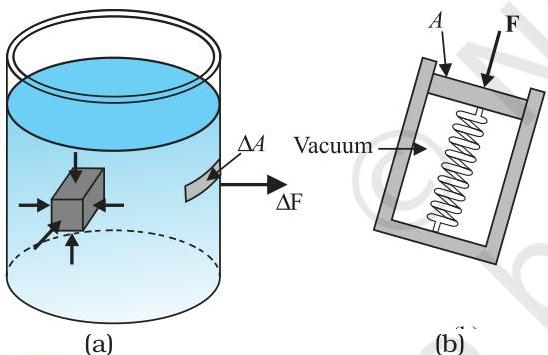 Fig. 9.1 (a) The force exerted by the liquid in the beaker on the submerged object or on the walls is normal (perpendicular) to the surface at all points.
(b) An idealised device for measuring pressure.
If $F$ represents the magnitude of this normal force acting on a piston of surface area $A$, then the average pressure, denoted $P_{av}$, is formally defined as the normal force distributed over that unit area.
$ P _ {a v} = \frac {F}{A} \tag {9.1} $
In principle, the piston's area can be reduced to an infinitesimally small size. In this limiting context, pressure is precisely defined as:
$ P = \lim _ {\Delta A \rightarrow 0} \frac {\Delta F}{\Delta A} \tag {9.2} $
Pressure is inherently a scalar physical quantity. It is important to reiterate that the numerator in Equations (9.1) and (9.2) refers specifically to the component of force perpendicular to the designated area, rather than the total (vector) force. Its fundamental dimensions are expressed as $\left[\mathrm{ML}^{-1}\mathrm{T}^{-2}\right]$. The standard SI unit for pressure is the newton per square meter ($\mathrm{Nm}^{-2}$), which is also designated as the pascal (Pa). This nomenclature honors the profound contributions of the French polymath Blaise Pascal (1623-1662), whose seminal investigations advanced the understanding of fluid pressure. Another frequently encountered unit of pressure is the atmosphere (atm), which represents the typical pressure exerted by the Earth's atmosphere at mean sea level (1 atm = 1.013 × 10^5 Pa).
An additional physical property, crucial for the comprehensive characterization of fluids, is density, symbolized by $\rho$. For a fluid possessing mass $m$ and occupying volume $V$,
$ \rho = \frac {m}{V} \tag {9.3} $
Density possesses dimensions of $\left[\mathrm{ML}^{-3}\right]$, and its standard SI unit is $\mathrm{kg~m}^{-3}$. This physical property is characterized as a positive scalar quantity. Liquids generally demonstrate significant incompressibility, which results in their density remaining approximately invariant across varying pressures. Conversely, gases manifest substantial fluctuations in density in response to changes in pressure.
Water's density at a temperature of $4^{\circ}\mathrm{C}$ (277 K) is quantified as $1.0 \times 10^{3} \mathrm{kg} \mathrm{m}^{-3}$. The relative density of any given substance is defined as the quotient of its own density and the density of water at $4^{\circ}\mathrm{C}$. This metric is a dimensionless, positive scalar value. For instance, aluminum has a relative density of 2.7, implying its absolute density is $2.7 \times 10^{3} \mathrm{kg} \mathrm{m}^{-3}$. A compilation of densities for several prevalent fluids is presented in Table 9.1.
Table 9.1 Densities of some common fluids at STP*
| Fluid | ρ (kg m-3) |
|---|---|
| Water | 1.00 × 10³ |
| Sea water | 1.03 × 10³ |
| Mercury | 13.6 × 10³ |
| Ethyl alcohol | 0.806 × 10³ |
| Whole blood | 1.06 × 10³ |
| Air | 1.29 |
| Oxygen | 1.43 |
| Hydrogen | 9.0 × 10⁻² |
| Interstellar space | ≈ 10-20 |
Example 9.1 Consider two thigh bones (femurs), each possessing a cross-sectional area of $10\mathrm{cm}^2$, which bear the weight of a human body's upper section, having a mass of 40 kg. Calculate the approximate average pressure experienced by these femurs.
Answer The combined cross-sectional area of both femurs is computed as $A = 2 \times 10 , \mathrm{cm}^2 = 20 \times 10^{-4} , \mathrm{m}^2$. The downward force exerted upon them is $F = 40 , \mathrm{kg} , \mathrm{wt} = 400 , \mathrm{N}$ (assuming $g = 10 , \mathrm{m} , \mathrm{s}^{-2}$). This force is oriented vertically downwards and therefore acts perpendicularly to the surfaces of the femurs. Consequently, the average pressure can be determined as:
$ P _ {\mathrm {a v}} = \frac {F}{A} = 2 \times 1 0 ^ {5} \mathrm {N m} ^ {- 2} $
9.2.1 Pascal's Law
The French scientist Blaise Pascal observed that the pressure within a fluid at rest remains constant at all points situated at the same height. This phenomenon can be demonstrated in a straightforward manner.
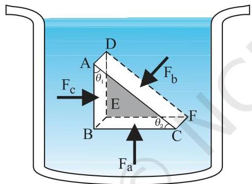 Fig. 9.2 Proof of Pascal's law. ABC-DEF is an element of the interior of a fluid at rest. This element is in the form of a right-angled prism. The element is small so that the effect of gravity can be ignored, but it has been enlarged for the sake of clarity.
Figure 9.2 illustrates a fluid element positioned within a static fluid. This specific element, denoted ABC-DEF, takes the form of a right-angled prism. Theoretically, this prismatic element is considered infinitesimally small, allowing every constituent part to be regarded as being at the same depth from the fluid surface, thereby ensuring that gravitational effects are uniform across all these points. However, for enhanced visual clarity, this element has been depicted in an enlarged state. The forces acting on this element originate from the surrounding fluid, and, as previously established, these forces must be oriented perpendicularly to the element's surfaces. Consequently, the fluid exerts pressures $P_{a}$, $P_{b}$, and $P_{c}$ on this element's areas, corresponding to the normal forces $F_{a}, F_{b}$, and $F_{c}$, respectively, as shown in Fig. 9.2 on faces BEFC, ADFC, and ADEB, which are designated as $A_{a}, A_{b}$, and $A_{c}$. Therefore,
$ F _ {\mathrm {b}} \sin \theta = F _ {\mathrm {c}}, \quad F _ {\mathrm {b}} \cos \theta = F _ {\mathrm {a}} \quad (\text {by equilibrium}) $
Geometrically, $A_{\mathrm{b}}\sin \theta = A_{\mathrm{c}}$ and $A_{\mathrm{b}}\cos \theta = A_{\mathrm{a}}$. Thus, by combining these relationships with the equilibrium conditions:
$ \frac {F _ {\mathrm {b}}}{A _ {\mathrm {b}}} = \frac {F _ {\mathrm {c}}}{A _ {\mathrm {c}}} = \frac {F _ {\mathrm {a}}}{A _ {\mathrm {a}}}; \quad P _ {b} = P _ {\mathrm {c}} = P _ {\mathrm {a}} \tag {9.4} $
This demonstrates that the pressure exerted within a fluid at rest is isotropic, meaning it is uniform in all directions. This outcome further underscores that, akin to other forms of stress, pressure fundamentally lacks vectorial properties, implying that no specific spatial direction can be ascribed to it. The force acting perpendicularly against any surface, whether internal or bounding, within a static fluid under pressure, is always normal to that surface, irrespective of the surface's orientation.
Next, let us consider a fluid element shaped as a horizontal bar of uniform cross-section. For this bar to be in equilibrium, the horizontal forces acting at its two extremities must be perfectly balanced, which necessitates that the pressure at these two ends be identical. This reasoning establishes that for a liquid in equilibrium, pressure is uniform across all points lying within a single horizontal plane. If, hypothetically, the pressure were not equal in different regions of the fluid, a net force would act upon it, initiating fluid flow. Therefore, in the absence of any fluid motion, the pressure throughout the fluid must be consistent across any given horizontal plane.
9.2.2 Variation of Pressure with Depth
Consider a fluid held static within a receptacle. As depicted in Fig. 9.3, point 1 is positioned at a vertical distance $h$ above point 2. The respective pressures at points 1 and 2 are denoted by $P_{1}$ and $P_{2}$. Let us isolate a cylindrical fluid element characterized by a base area $A$ and height $h$. Given that the fluid is in equilibrium, the net horizontal forces must be zero, and the net vertical forces must precisely counteract the element's weight. The forces operating in the vertical dimension comprise the downward force exerted by the fluid pressure at the top $(P_{1}A)$ and the upward force from the fluid pressure at the bottom $(P_{2}A)$. If $mg$ represents the weight of the fluid within this cylindrical volume, we can establish the following relationship:
$ \left(P _ {2} - P _ {1}\right) A = m g \tag {9.5} $
Subsequently, if $\rho$ signifies the mass density of the fluid, the mass of the fluid can be expressed as $m = \rho V = \rho hA$. Substituting this into the previous equation yields:
$ P _ {2} - P _ {1} = \rho g h \tag {9.6}
$
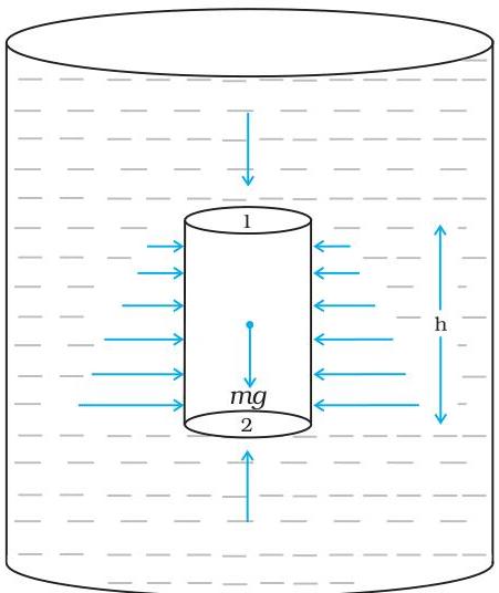 Fig.9.3 Fluid under gravity. The effect of gravity is illustrated through pressure on a vertical cylindrical column.
The observed pressure differential is contingent upon the vertical separation $h$ between the two points (1 and 2), the mass density $\rho$ of the fluid, and the acceleration due to gravity $g$. Should point 1 be relocated to the uppermost surface of the fluid (e.g., water), which is exposed to the atmosphere, $P_1$ can be substituted with the atmospheric pressure $(P_a)$, and $P_2$ can be replaced by $P$. Equation (9.6) then transforms into:
$ P = P _ {a} + \rho g h \tag {9.7} $
Consequently, the pressure $P$ at a specific depth below the surface of a liquid exposed to the atmosphere exceeds the atmospheric pressure by a quantity $\rho gh$. This incremental pressure, $P - P_{a}$, at depth $h$ is defined as the gauge pressure at that particular location.
It is noteworthy that the cross-sectional area of the cylinder does not appear in the formulation for absolute pressure presented in Eq. (9.7). This implies that the vertical extent of the fluid column is the crucial factor, rather than its cross-sectional or base area, or the overall shape of the container. Furthermore, the liquid pressure remains uniform at all points situated at the same horizontal plane (i.e., identical depth). This principle is effectively demonstrated by the hydrostatic paradox. Consider three containers, A, B, and C [Fig.9.4], each possessing a distinct shape. These vessels are interconnected at their base by a horizontal conduit. Upon being filled with water, the liquid level in all three containers is observed to be identical, despite the differing volumes of water each vessel accommodates. This phenomenon occurs because the water at the base exerts the same pressure beneath each segment of the vessel.
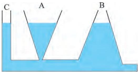 Fig 9.4 Illustration of hydrostatic paradox. The three vessels $A$, $B$ and $C$ contain different amounts of liquids, all upto the same height.
Example 9.2 What is the pressure on a swimmer $10\mathrm{m}$ below the surface of a lake?
$h = 10\mathrm{m}$ and $\rho = 1000\mathrm{kg}\mathrm{m}^{-3}$. Take $\mathrm{g} = 10\mathrm{ms}^{-2}$. Given these parameters, the pressure can be calculated using Eq. (9.7) as follows:
$ \begin{array}{l} P = P _ {0} + \rho g h \ = 1. 0 1 \times 1 0 ^ {5} \mathrm {P a} + 1 0 0 0 \mathrm {k g m} ^ {- 3} \times 1 0 \mathrm {m s} ^ {- 2} \times 1 0 \mathrm {m} \ = 2. 0 1 \times 1 0 ^ {5} \mathrm {P a} \ = 2 \mathrm {a t m} \ \end{array} $
This represents a 100% increment in pressure relative to the surface level. Notably, at a depth of $1\mathrm{km}$, the pressure increase is a substantial 100 atm. Submarines are engineered to endure such immense pressures.
9.2.3 Atmospheric Pressure and Gauge Pressure
Atmospheric pressure at any given point is quantitatively defined as the force exerted by the column of air of unit cross-sectional area extending vertically from that point to the uppermost boundary of the atmosphere. At mean sea level, this pressure typically measures $1.013 \times 10^{5} \mathrm{~Pa}$, which is equivalent to 1 standard atmosphere. The pioneering methodology for measuring atmospheric pressure was developed by the Italian scientist Evangelista Torricelli (1608-1647). His apparatus, illustrated in Fig. 9.5 (a), involves a long glass tube, sealed at one end and completely filled with mercury, which is then inverted into a trough also containing mercury. This instrument is commonly known as a 'mercury barometer'. The void space above the mercury column within the tube contains only mercury vapor, whose pressure $P$ is so minimal that it can be considered negligible. Consequently, the pressure at Point A is effectively zero. For hydrostatic equilibrium, the pressure inside the column at Point B must precisely match the external atmospheric pressure, $\mathrm{P}_{a}$, observed at Point C.
$ P_{a} = \rho gh \tag{9.8} $
In this equation, $\rho$ denotes the density of the mercury, and $h$ represents the vertical height of the mercury column within the tube.
Empirical observations from this experiment reveal that at sea level, the mercury column in the barometer attains a height of approximately 76 cm, which corresponds to one atmosphere (1 atm). This value can also be derived by substituting the appropriate density value for mercury into Eq. (9.8). Pressure is frequently expressed using units referencing the height of a mercury column, such as cm or mm of mercury (Hg). A pressure equivalent to 1 mm of mercury is designated as a torr, named after Torricelli.
1 torr = 133 Pa
The units of mm of Hg and torr are particularly employed in medicine and physiology. In the field of meteorology, the bar and millibar are established as prevalent units of pressure.
1 bar = 10⁵ Pa
An open-tube manometer serves as an effective instrument for quantifying pressure differentials. This apparatus comprises a U-shaped tube containing an appropriate fluid; a low-density liquid (e.g., oil) is employed for resolving minor pressure variations, while a high-density liquid (e.g., mercury) is utilized for substantial pressure discrepancies. One aperture of the tube remains exposed to the ambient atmosphere, whereas the opposing aperture is interfaced with the system whose pressure is to be ascertained [refer to Fig. 9.5 (b)]. The pressure P at point A is equivalent to the pressure observed at point B. The quantity typically measured is the gauge pressure, defined as $P - P_s$, which can be derived from Eq. (9.8) and exhibits direct proportionality to the height $h$ of the manometric fluid column.
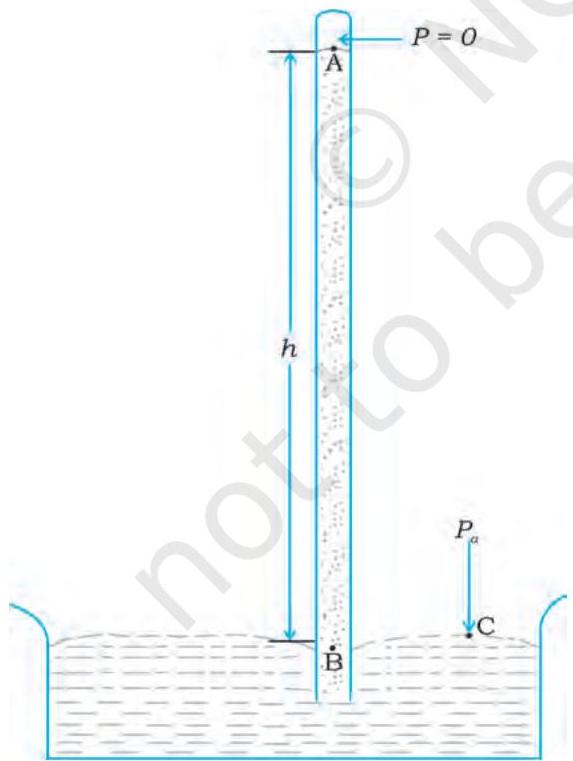 Fig 9.5 (a) The mercury barometer.
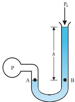 (b) The open tube manometer
Fig 9.5 Two pressure measuring devices.
(b) The open tube manometer
Fig 9.5 Two pressure measuring devices.
Within a fluid-filled U-tube, the pressure at any given horizontal level is uniform across both limbs. For liquids, density exhibits negligible variation across significant fluctuations in pressure and temperature, allowing for its reliable assumption as a constant in the current context. Conversely, gases demonstrate substantial density changes in response to alterations in pressure and temperature. Consequently, liquids are predominantly regarded as incompressible, a characteristic not shared by gases.
Example 9.3 The density of the atmosphere at sea level is 1.29 kg/m³. Assume that it does not change with altitude. Then how high would the atmosphere extend?
Solution Applying Equation (9.7):
$ \rho g h = 1.29 \mathrm{kg} \mathrm{m}^{-3} \times 9.8 \mathrm{m s}^{-2} \times h \mathrm{m} = 1.01 \times 10^{5} \mathrm{Pa} $
$ \therefore h = 7989 \mathrm{m} \approx 8 \mathrm{km} $
In actual atmospheric conditions, air density diminishes progressively with increasing altitude. Concurrently, the gravitational acceleration 'g' also experiences a reduction. The Earth's atmospheric cover extends beyond 100 km, characterized by a continuous decline in pressure. Furthermore, it is pertinent to recognize that the atmospheric pressure at sea level does not consistently register at 760 mm of mercury. A decrease of 10 mm or greater in the mercury column frequently indicates the imminent arrival of stormy weather.
Example 9.4 At a depth of 1000 m in an ocean (a) what is the absolute pressure? (b) What is the gauge pressure? (c) Find the force acting on the window of area 20 cm × 20 cm of a submarine at this depth, the interior of which is maintained at sea-level atmospheric pressure. (The density of sea water is 1.03 × 10³ kg m⁻³, g = 10 m s⁻².)
Solution Given: $h = 1000,\mathrm{m}$ and $\rho = 1.03 \times 10^{3},\mathrm{kg},\mathrm{m}^{-3}$.
(a) The absolute pressure, derived from Equation (9.6), is calculated as:
$ \begin{array}{l} P = P_{\mathrm{atm}} + \rho g h \ = 1.01 \times 10^{5} ,\mathrm{Pa} \ \quad + 1.03 \times 10^{3} ,\mathrm{kg} ,\mathrm{m}^{-3} \times 10,\mathrm{m} ,\mathrm{s}^{-2} \times 1000,\mathrm{m} \ = 104.01 \times 10^{5} ,\mathrm{Pa} \ \approx 104,\mathrm{atm} \end{array} $
(b) The gauge pressure is determined by the difference $P - P_{\mathrm{atm}}$, which simplifies to $\rho g h$. This value is then represented as $P_{\mathrm{g}}$:
$ \begin{array}{l} P_{\mathrm{g}} = 1.03 \times 10^{3} ,\mathrm{kg} ,\mathrm{m}^{-3} \times 10,\mathrm{m},\mathrm{s}^{-2} \times 1000,\mathrm{m} \ = 103 \times 10^{5} ,\mathrm{Pa} \ \approx 103,\mathrm{atm} \end{array} $
(c) The external pressure acting on the submarine is $P = P_{\mathrm{atm}} + \rho g h$, while the internal pressure is maintained at $P_{\mathrm{atm}}$ (sea-level atmospheric pressure). Consequently, the net pressure differential across the window is the gauge pressure, $P_{\mathrm{g}} = \rho g h$. Given the window's area $A = 0.04,\mathrm{m}^2$, the resultant force exerted upon it is:
$ F = P_{\mathrm{g}} A = 103 \times 10^{5} ,\mathrm{Pa} \times 0.04,\mathrm{m}^{2} = 4.12 \times 10^{5} ,\mathrm{N} $
9.2.4 Hydraulic Machines
Let's investigate the effects of altering the pressure on a fluid within an enclosed container. Imagine a horizontal cylinder equipped with a piston and three vertical standpipes positioned at various intervals [Fig. 9.6 (a)]. The liquid column height in these vertical tubes serves as an indicator of the pressure within the horizontal cylinder. This pressure is inherently uniform across all points. Should the piston be advanced, the liquid level in all tubes will ascend, subsequently stabilizing at an identical elevation in each.
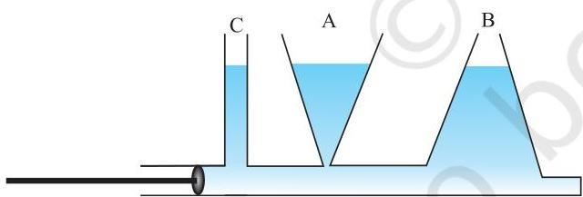 Fig 9.6 (a) Whenever external pressure is applied on any part of a fluid in a vessel, it is equally transmitted in all directions.
This observation reveals that an augmentation of pressure within the cylinder results in its uniform dissemination throughout the fluid. Consequently, it can be asserted that any external pressure exerted upon a portion of a fluid enclosed within a container is propagated without reduction and with equal intensity in all orientations. This principle constitutes an alternative formulation of Pascal's Law, which finds extensive utility in various everyday contexts.
Numerous mechanisms, including hydraulic lifts and hydraulic braking systems, operate on the foundation of Pascal's law. Within these systems, liquids serve as the medium for pressure transmission. Considering a hydraulic lift, as depicted in Fig. 9.6 (b), two pistons are demarcated by a liquid-filled chamber. A piston possessing a smaller cross-sectional area, $A_{1}$, is employed to apply a force, $F_{1}$, directly onto the liquid. The resultant pressure, $P = \frac{F_{1}}{A_{1}}$, is then propagated uniformly throughout the liquid to the larger cylinder, which is fitted with a larger piston of area $A_{2}$. This propagation generates an upward force equivalent to $P \times A_{2}$. Consequently, this larger piston can sustain a substantial force (e.g., the considerable weight of a vehicle like a car or truck positioned on the platform), denoted as $F_{2} = PA_{2} = \frac{F_{1}A_{2}}{A_{1}}$. Adjusting the force applied at $A_{1}$ allows for the vertical displacement of the platform. Hence, the initial force has been amplified by a factor of $\frac{A_{2}}{A_{1}}$, which represents the mechanical advantage inherent to this apparatus. The subsequent example elucidates this concept.
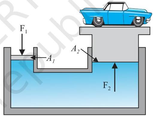 Fig 9.6 (b) Schematic diagram illustrating the principle behind the hydraulic lift, a device used to lift heavy loads.
Example 9.5 Illustrative Problem 9.5: Consider two syringes of dissimilar cross-sectional areas (excluding their needles), both filled with water and interconnected by a snugly fitted, water-filled rubber tubing. The diameters of the smaller and larger pistons measure $1.0,\mathrm{cm}$ and $3.0,\mathrm{cm}$, respectively. (a) Determine the magnitude of the force exerted on the larger piston when a force of $10,\mathrm{N}$ is applied to the smaller piston. (b) If the smaller piston is depressed by $6.0,\mathrm{cm}$, calculate the corresponding outward displacement of the larger piston.
Answer (a) Solution (a): Given that pressure is conveyed without attenuation across the entire fluid,
$
\begin{array}{l} F_{2} = \frac{A_{2}}{A_{1}} F_{1} = \frac{\pi (3 / 2 \times 10^{-2} \mathrm{m})^{2}}{\pi (1 / 2 \times 10^{-2} \mathrm{m})^{2}} \times 10 \mathrm{N} \ = 90 \mathrm{N} \end{array} $
(b) Assuming water to be perfectly incompressible, the volumetric displacement caused by the inward motion of the smaller piston precisely corresponds to the outward volumetric displacement generated by the larger piston.
$ \begin{array}{l} L_{1} A_{1} = L_{2} A_{2} \ L_{2} = \frac{A_{1}}{A_{2}} L_{1} = \frac{\pi (1 / 2 \times 10^{-2} \mathrm{m})^{2}}{\pi (3 / 2 \times 10^{-2} \mathrm{m})^{2}} \times 6 \times 10^{-2} \mathrm{m} \ \simeq 0.67 \times 10^{-2} \mathrm{m} = 0.67 \mathrm{cm} \end{array} $
It should be noted that atmospheric pressure is uniformly applied to both pistons and has therefore been disregarded in this calculation.
Example 9.6 Consider a car lift where compressed air applies a force $F_{1}$ to a smaller piston with a radius of $5.0 , \text{cm}$. This pressure is subsequently conveyed to a larger piston, which possesses a radius of $15 , \text{cm}$ (Fig 9.7). Given that the vehicle intended for lifting has a mass of $1350 , \text{kg}$, determine the magnitude of $F_{1}$. Furthermore, what is the required pressure to achieve this lifting operation? (Assume $g = 9.8 , \text{ms}^{-2}$).
Answer Given that pressure propagates uniformly and without reduction throughout the fluid medium.
$ \begin{array}{l} F_{1} = \frac{A_{1}}{A_{2}} F_{2} = \frac{\pi (5 \times 10^{-2} \mathrm{m})^{2}}{\pi (15 \times 10^{-2} \mathrm{m})^{2}} (1350 , \mathrm{kg} \times 9.8 , \mathrm{ms}^{-2}) \ = 1470 , \mathrm{N} \ \approx 1.5 \times 10^{3} , \mathrm{N} \end{array} $
The pneumatic pressure necessary to generate this force is calculated as follows:
$ P = \frac{F_{1}}{A_{1}} = \frac{1.5 \times 10^{3} , \mathrm{N}}{\pi (5 \times 10^{-2})^{2} , \mathrm{m}} = 1.9 \times 10^{5} , \mathrm{Pa} $
This value approaches approximately twice the typical atmospheric pressure.
Automotive hydraulic braking systems operate on an identical fundamental principle. Upon the application of a modest force to the pedal by the driver's foot, the master piston is displaced within the master cylinder. The resultant pressure generated is then conveyed via the brake fluid to exert force upon a piston of greater surface area. Consequently, a substantial force is applied to this piston, causing it to move and expand the brake shoes against the brake lining. This mechanism effectively translates a minimal input force on the pedal into a significant retarding force acting upon the wheel. A notable benefit of this arrangement lies in the uniform transmission of the pressure, established by depressing the pedal, to all brake cylinders associated with the four wheels, thereby ensuring an equitable braking effort across the entire vehicle.
9.3 STREAMLINE FLOW
Our preceding discussions have focused on quiescent fluids. The analysis of fluids undergoing motion constitutes the field of fluid dynamics. When a water faucet is gradually opened, the initial discharge exhibits laminar characteristics, yet this smooth behavior dissipates as the efflux velocity intensifies. In examining fluid motion, our primary concern is the behavior of individual fluid particles at a specific spatial location at a given temporal instant. Fluid flow is designated as steady if, at any designated point, the velocity of each successive fluid particle traversing that point maintains temporal constancy. It is crucial to note that this condition does not imply uniform velocity across distinct spatial points. An individual particle's velocity may indeed alter as it progresses from one location to another. Specifically, at a subsequent point, the particle might possess a different velocity, but all subsequent particles passing through that second point will replicate the precise kinematic behavior of the particle that immediately preceded them. Each particle traverses an unperturbed trajectory, and these individual particle paths remain distinct, never intersecting.
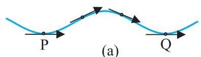
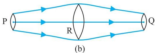 Fig. 9.7 The meaning of streamlines. (a) A typical trajectory of a fluid particle. (b) A region of streamline flow.
Within a steady flow regime, the trajectory traced by a fluid particle is designated as a streamline. This is formally characterized as a curve such that its tangent at any arbitrary point corresponds precisely to the direction of the fluid velocity at that specific point. Examining the particle's trajectory depicted in Fig. 9.7 (a), this curve illustrates the temporal progression of a fluid particle's motion. The segment PQ effectively serves as a persistent graphical representation of the fluid's movement, delineating its streaming pattern. A fundamental property dictates that
no two streamlines can intersect; should they do so, an approaching fluid particle would face an indeterminate choice of path, thereby violating the condition of steady flow. Consequently, under steady flow conditions, the configuration of these flow lines remains invariant over time. The question then arises: how are streamlines drawn with sufficient density? If one were to depict a streamline for every individual flowing particle, the result would be an undifferentiated continuum of lines. Instead, consider conceptual planes oriented perpendicularly to the fluid's direction of motion, for instance, at the three points P, R, and Q illustrated in Fig. 9.7 (b). These planar sections are judiciously chosen such that their perimeters are delineated by the identical set of streamlines. This implies that the quantity of fluid particles traversing the surfaces indicated at P, R, and Q remains constant. If the cross-sectional areas at these respective points are denoted as $A_{\mathrm{P}}, A_{\mathrm{R}}$, and $A_{\mathrm{Q}}$, and the corresponding fluid particle speeds are $\nu_{\mathrm{P}}, \nu_{\mathrm{R}}$, and $\nu_{\mathrm{Q}}$, then the mass of fluid $\Delta m_{\mathrm{p}}$ passing through $A_{\mathrm{P}}$ during a brief time interval $\Delta t$ is given by $\rho_{\mathrm{P}} A_{\mathrm{P}} \nu_{\mathrm{P}} \Delta t$. Analogously, the mass of fluid $\Delta m_{\mathrm{R}}$ traversing $A_{\mathrm{R}}$ within the same interval $\Delta t$ is $\rho_{\mathrm{R}} A_{\mathrm{R}} \nu_{\mathrm{R}} \Delta t$, and similarly, the mass of fluid $\Delta m_{\mathrm{Q}}$ crossing $A_{\mathrm{Q}}$ is $\rho_{\mathrm{Q}} A_{\mathrm{Q}} \nu_{\mathrm{Q}} \Delta t$. The principle of conservation of mass dictates that the mass of liquid exiting any given volume must equal the mass entering it, universally applicable. Therefore,
$ \rho_ {\mathrm {P}} A _ {\mathrm {P}} v _ {\mathrm {P}} \Delta t = \rho_ {\mathrm {R}} A _ {\mathrm {R}} v _ {\mathrm {R}} \Delta t = \rho_ {\mathrm {Q}} A _ {\mathrm {Q}} v _ {\mathrm {Q}} \Delta t \tag {9.9} $
When considering the movement of incompressible fluids,
$ \rho_ {\mathrm {P}} = \rho_ {\mathrm {R}} = \rho_ {\mathrm {Q}} $
Consequently, Equation (9.9) simplifies to
$ A _ {\mathrm {P}} v _ {\mathrm {P}} = A _ {\mathrm {R}} v _ {\mathrm {R}} = A _ {\mathrm {Q}} v _ {\mathrm {Q}} \tag {9.10} $
This relationship is known as the continuity equation, representing the principle of mass conservation for incompressible fluid flows. More broadly,
$ A v = \text {constant} \tag {9.11} $
The product $Av$ represents the volumetric flow rate, which maintains a constant value across the entire flow conduit. Therefore, in regions where the pipe narrows and streamlines converge, the fluid velocity increases, and conversely, it decreases in wider sections. As depicted in (Fig 9.7b), given that $A_{\mathrm{R}} > A_{\mathrm{Q}}$ implies $\nu_{\mathrm{R}} < \nu_{\mathrm{Q}}$, the fluid undergoes acceleration as it transitions from point R to point Q. This change in velocity is linked to a corresponding alteration in pressure within horizontal fluid conduits.
Laminar flow conditions prevail at modest fluid velocities. However, upon exceeding a specific threshold, termed the critical speed, the flow ceases to be steady and transitions into a turbulent state. A common illustration of this phenomenon is observed when a rapidly moving river current encounters obstructions such as rocks, leading to the formation of small, frothy, swirling areas known as 'white water rapids'.
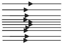
The flow patterns for various fluid movements are illustrated by streamlines in Figure 9.8. For instance, panel (a) of Fig. 9.8 depicts a laminar flow regime, characterized by fluid velocities that may vary in magnitude across different points
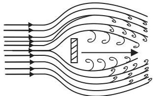
but their directions remain parallel. Panel (b) of Figure 9.8 presents a representation of turbulent flow.
 (a)
(a)
 (b)
Fig. 9.8 (a) Some streamlines for fluid flow. (b) A jet of air striking a flat plate placed perpendicular to it. This is an example of turbulent flow.
(b)
Fig. 9.8 (a) Some streamlines for fluid flow. (b) A jet of air striking a flat plate placed perpendicular to it. This is an example of turbulent flow.
9.4 BERNOULLI'S PRINCIPLE
Although fluid dynamics is an intricate field, the principle of energy conservation allows us to deduce valuable characteristics for flows that are steady or laminar.
Consider a fluid traversing a conduit with varying cross-sectional areas and elevations, as depicted in Fig. 9.9. Assuming a steady flow of an incompressible fluid through this pipe, its velocity must necessarily change according to the continuity equation. This acceleration necessitates the application of a force, which originates from the surrounding fluid, implying that pressure must differ across various regions. Bernoulli's equation provides a comprehensive relationship connecting the pressure differential between any two points within a pipe to both alterations in velocity (representing kinetic energy changes) and variations in elevation (representing potential energy changes). This fundamental relationship was formulated by the Swiss physicist Daniel Bernoulli in 1738.
Let's examine the fluid movement between two distinct regions, specifically region 1 (denoted as BC) and region 2 (denoted as DE). Imagine a fluid element initially situated between points B and D. Over an infinitesimal time interval $\Delta t$, this fluid element will have undergone displacement. If $\nu_{1}$ represents the fluid speed at B and $\nu_{2}$ at D, then the fluid originally at B will have advanced a distance $\nu_{1}\Delta t$ to point C (where $\nu_{1}\Delta t$ is sufficiently small to assume a constant cross-section along BC). Concurrently, during the same interval $\Delta t$, the fluid initially at D will move to E, covering a distance equivalent to $\nu_{2}\Delta t$. Pressures $P_{1}$ and $P_{2}$ exert forces on the planar surfaces of areas $A_{1}$ and $A_{2}$ that define these two regions, as illustrated. The work performed on the fluid at the left boundary (BC) is given by $W_{1} = P_{1}A_{1}(\nu_{1}\Delta t) = P_{1}\Delta V$. Due to the principle of continuity, the same volume $\Delta V$ passes through both regions. Consequently, the work done by the fluid at the other boundary (DE) is $W_{2} = P_{2}A_{2}(\nu_{2}\Delta t) = P_{2}\Delta V$. Alternatively, the work done on the fluid at this end is $-P_{2}\Delta V$. Therefore, the net work executed on the fluid is
$ W _ {1} - W _ {2} = \left(P _ {1} - P _ {2}\right) \Delta V $
This work is partitioned into two components: one contributing to the modification of the fluid's kinetic energy, and the other to the alteration of its gravitational potential energy. If $\rho$ denotes the fluid's density, and $\Delta m = \rho A_1 v_1 \Delta t = \rho \Delta V$ represents the mass of fluid flowing through the pipe during the time $\Delta t$, then the corresponding change in gravitational potential energy is
$ \Delta U = \rho g \Delta V (h _ {2} - h _ {1}) $
The concomitant change in its kinetic energy is expressed as
$ \Delta K = \frac {1}{2} \rho \Delta V (v _ {2} ^ {2} - v _ {1} ^ {2}) $
By applying the work-energy theorem (as discussed in Chapter 6) to this specific volume of fluid, we arrive at the following relation:
$ \left(P _ {1} - P _ {2}\right) \Delta V = \frac {1}{2} \rho \Delta V \left(v _ {2} ^ {2} - v _ {1} ^ {2}\right) + \rho g \Delta V \left(h _ {2} - h _ {1}\right) $
Dividing each term of the equation by $\Delta V$ yields
$ \left(P _ {1} - P _ {2}\right) = \frac {1}{2} \rho \left(v _ {2} ^ {2} - v _ {1} ^ {2}\right) + \rho g \left(h _ {2} - h _ {1}\right) $
Rearranging the terms presented above leads to
$ P _ {1} + \frac {1}{2} \rho v _ {1} ^ {2} + \rho g h _ {1} = P _ {2} + \frac {1}{2} \rho v _ {2} ^ {2} + \rho g h _ {2} \tag {9.12} $
This relationship is known as Bernoulli's equation. Given that subscripts 1 and 2 denote arbitrary points within the flow path, the general form of this expression can be stated as:
$ P + \frac {1}{2} \rho v ^ {2} + \rho g h = \text {constant} \tag {9.13} $
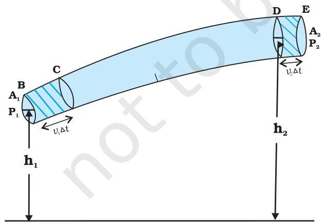 Fig. 9.9 Depiction of ideal fluid flow through a conduit with a changing cross-sectional area. The fluid segment of length $v_{1}\Delta t$ displaces into the segment of length $v_{2}\Delta t$ over the time interval $\Delta t$.
Expressed verbally, Bernoulli's principle asserts that along any given streamline, the aggregate of the static pressure $(P)$, the kinetic energy per unit volume $\left(\frac{\rho v^2}{2}\right)$, and the potential energy per unit volume $(\rho gh)$ maintains an invariant value.
It is crucial to recognize that the application of the energy conservation principle within this context presumes the absence of energy dissipation caused by frictional forces. However, in reality, fluid motion invariably involves some degree of energy loss attributable to internal friction. This phenomenon occurs because distinct layers within the fluid stream move at varying velocities, leading to the exertion of shear forces between them, which, in turn, results in energy degradation. This intrinsic characteristic of a fluid is termed viscosity, a concept that will be elaborated upon further in a subsequent discussion. The kinetic energy thus dissipated from the fluid system is transformed into thermal energy. Consequently, Bernoulli's equation is most accurately applicable to fluids exhibiting negligible viscosity, often referred to as non-viscous fluids. A further prerequisite for the valid application of Bernoulli's theorem is that the fluids must be incompressible, as their inherent elastic energy is not factored into the equation. Despite these theoretical limitations, the principle finds extensive practical utility, enabling the elucidation of diverse phenomena in fluids characterized by low viscosity and incompressibility. Furthermore, Bernoulli's equation is not valid for non-steady or turbulent flow regimes, owing to the continuous temporal fluctuations in both velocity and pressure inherent to such conditions.
In a scenario where a fluid is static, meaning its velocity is uniformly zero throughout, Bernoulli's equation simplifies to:
$ P _ {1} + \rho g h _ {1} = P _ {2} + \rho g h _ {2} $
$ \left(P _ {1} - P _ {2}\right) = \rho g \left(h _ {2} - h _ {1}\right) $
This result is identical to Eq. (9.6).
9.4.1 Speed of Efflux: Torricelli's Law
Efflux refers to the outward flow of a fluid. Torricelli observed that the velocity at which fluid exits an open reservoir is described by an equation identical in form to that governing a freely falling object. Consider a reservoir holding a liquid of density $\rho$, featuring a small aperture on its side positioned at a height $y_1$ from its base (refer to Fig. 9.10). The air situated above the liquid surface, which is at height $y_2$, exerts a pressure $P$. Based on the principle of continuity, as expressed in Eq. (9.10), we have:
$ v _ {1} A _ {1} = v _ {2} A _ {2} $
$ v _ {2} = \frac {A _ {1}}{A _ {2}} v _ {1} $
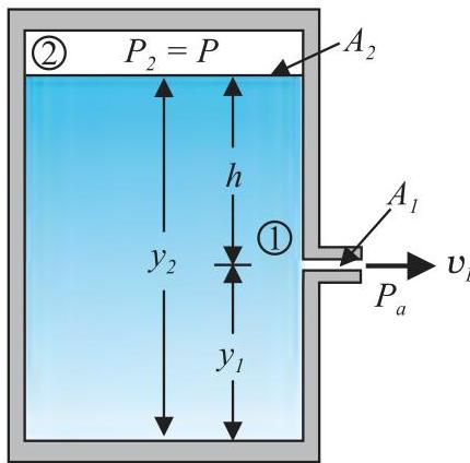 Fig. 9.10 Torricelli's law. The speed of efflux, $v_1$ , from the side of the container is given by the application of Bernoulli's equation. If the container is open at the top to the atmosphere then $v_1 = \sqrt{2gh}$ .
Should the reservoir's cross-sectional area $A_2$ significantly surpass that of the aperture $(A_2 \gg A_1)$, the fluid at the upper surface can be considered approximately stationary, implying $v_2 = 0$. Now, by applying Bernoulli's equation to points 1 and 2, and recognizing that at the aperture, $P_1 = P_a$ (the ambient atmospheric pressure), we derive from Eq. (9.12):
$ P _ {a} + \frac {1}{2} \rho v _ {1} ^ {2} + \rho g y _ {1} = P + \rho g y _ {2} $
Defining $h$ as the vertical distance $y_2 - y_1$, the expression becomes:
$ v _ {1} = \sqrt {2 g h + \frac {2 (P - P _ {a})}{\rho}} \tag {9.14} $
In scenarios where $P \gg P_a$ and the term $2gh$ is negligible, the efflux velocity is predominantly governed by the internal pressure of the container. This condition is exemplified in applications such as rocket propulsion. Conversely, if the container is exposed to the atmosphere, then $P = P_a$, which simplifies the equation to:
$ v _ {1} = \sqrt {2 g h} \tag {9.15} $
This outcome is precisely the velocity attained by an object in free fall. Equation (9.15) encapsulates Torricelli's law.
9.4.2 Dynamic Lift
Dynamic lift refers to the resultant force exerted on an object, such as an aircraft wing, a hydrofoil, or a rotating sphere, as a consequence of its movement within a fluid medium. Observations in various sports, including cricket, tennis, baseball, and golf, reveal that a spinning ball departs from its expected parabolic flight path through the air. This observed deflection can be partially attributed to the principles of Bernoulli's theorem.
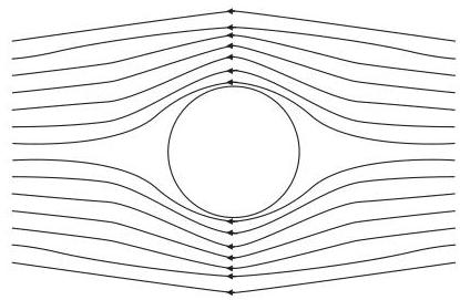
(i) Non-rotating Ball Movement: As depicted in Fig. 9.11(a), the streamlines enveloping a non-spinning ball traversing a fluid exhibit symmetry. This symmetrical flow pattern indicates that the fluid's (air's) velocity at equivalent positions above and below the ball is identical, leading to an absence of pressure differential. Consequently, the air imparts no net vertical force, either upward or downward, upon the ball.
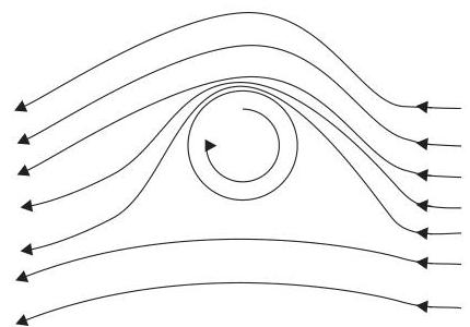
(ii) Ball Movement with Rotation: A rotating ball entrains a layer of air in its immediate vicinity; a rougher surface amplifies this air entrainment. Figure 9.11(b) illustrates the airflow streamlines for a ball simultaneously translating and rotating. As the ball progresses forward, the air relative to the ball moves backward. This interaction causes the air velocity above the ball, relative to its surface, to increase, while the velocity below it decreases (refer to Section 9.3). Consequently, the streamlines become denser above the ball and more dispersed beneath it. This disparity in air velocities generates a pressure differential between the lower and upper surfaces, resulting in a net upward force on the ball. This phenomenon of dynamic lift, induced by rotation, is termed the Magnus effect.
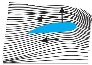
Aerofoil Design and Aircraft Wing Lift: Figure 9.11(c) presents an aerofoil, which is a specifically contoured solid component engineered to generate an upward dynamic lift as it traverses horizontally through an air mass. The typical cross-sectional profile of an aircraft's wing resembles the aerofoil depicted in Fig. 9.11(c), complete with its surrounding streamlines. As the aerofoil advances into the airstream, its angular disposition relative to the flow vector induces a greater concentration of streamlines above the wing compared to those beneath it. This results in a higher airflow velocity over the upper surface than beneath the lower surface. Consequently, an upward force is produced, manifesting as dynamic lift on the wings, which serves to counteract the aircraft's gravitational weight. The subsequent example provides a practical demonstration of this principle.
 (a)
(a)
 (b)
(b)
 (c)
Fig 9.11 (a) Fluid streaming past a static sphere. (b) Streamlines for a fluid around a sphere spinning clockwise. (c) Air flowing past an aerofoil.
(c)
Fig 9.11 (a) Fluid streaming past a static sphere. (b) Streamlines for a fluid around a sphere spinning clockwise. (c) Air flowing past an aerofoil.
Example 9.7 A fully loaded Boeing aircraft has a mass of $3.3 \times 10^{5} , \mathrm{kg}$. Its total wing area is $500 , \mathrm{m}^{2}$. It is in level flight with a speed of $960 , \mathrm{km/h}$. (a) Estimate the pressure difference between the lower and upper surfaces of the wings (b) Estimate the fractional increase in the speed of the air on the upper surface of the wing relative to the lower surface. [The density of air is $\rho = 1.2 , \mathrm{kg} , \mathrm{m}^{-3}$]
(a) The upward force generated by the pressure disparity effectively counteracts the weight of the Boeing aircraft.
$ \begin{array}{l} \Delta P \ A = 3.3 \times 10^{5} , \mathrm{kg} \times 9.8 \ \Delta P = (3.3 \times 10^{5} , \mathrm{kg} \times 9.8 , \mathrm{m} , \mathrm{s}^{-2}) / 500 , \mathrm{m}^{2} \ = 6.5 \times 10^{3} , \mathrm{Nm}^{-2} \end{array} $
(b) For the subsequent analysis, the minor variation in height between the upper and lower surfaces, as referenced in Eq. (9.12), is considered negligible. Consequently, the pressure differential between these surfaces is given by:
$ \Delta P = \frac{\rho}{2} \left(v_{2}^{2} - v_{1}^{2}\right) $
Here, $v_{2}$ denotes the velocity of the airflow across the upper aerofoil surface, while $v_{1}$ represents the airflow velocity beneath the lower surface.
$ (v_{2} - v_{1}) = \frac{2 \Delta P}{\rho (v_{2} + v_{1})} $
By considering the mean velocity
$ \begin{array}{l} v_{av} = (v_{2} + v_{1}) / 2 = 960 , \mathrm{km/h} = 267 , \mathrm{m} , \mathrm{s}^{-1}, \ \text{we have} \end{array} $
$ (v_{2} - v_{1}) / v_{av} = \frac{\Delta P}{\rho v_{av}^{2}} \approx 0.08 $
It is determined that the airflow velocity over the wing's upper surface is required to be merely 8% greater than that beneath it.
9.5 VISCOSITY
Unlike ideal fluids, most real fluids exhibit a certain opposition to flow. This impedance to fluid movement manifests as an internal friction, conceptually akin to the frictional forces encountered when a solid object glides over a surface; it is termed viscosity. This inherent resistive force arises specifically when there is differential motion between adjacent strata of a liquid. Consider, for instance, a fluid such as oil contained between two glass plates, as depicted in Fig. 9.12 (a). If the lower plate remains static while the upper plate is propelled at a constant velocity $\mathbf{v}$ relative to the stationary one, a force is required. Should honey be substituted for oil, a larger force would be necessary to achieve the identical plate velocity, thus indicating that honey possesses a higher viscosity than oil. A fundamental principle dictates that the fluid layer immediately adjacent to a solid boundary adopts the velocity of that boundary. Consequently, the liquid layer in contact with the upper surface attains a velocity of $\mathbf{v}$, whereas the layer touching the fixed lower surface remains immobile. The velocities of intermediate layers exhibit a linear progression, increasing uniformly from zero at the bottom layer to $\mathbf{v}$ at the uppermost layer. Within this velocity gradient, each liquid layer experiences a forward drag from the layer above it and a backward drag from the layer beneath it, generating forces between these layers. This particular mode of flow is designated as laminar. In this regime, the fluid strata glide smoothly past one another, much like the individual pages of a book when it lies flat on a surface and a tangential force is applied to its uppermost cover. In the context of fluid transport through a conduit or tube, the velocity of the liquid layer is maximal along the central axis of the tube and progressively diminishes as one approaches the confining walls, ultimately reaching zero at the boundary, as illustrated in Fig. 9.12 (b). Importantly, the velocity maintains a constant value across any given cylindrical surface concentric with the tube's axis.
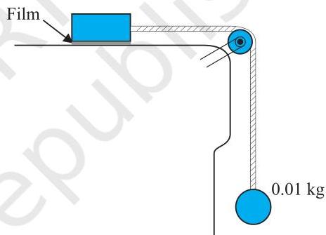 Fig. 9.12 (a) A fluid layer positioned between two parallel glass plates, where the bottom plate remains stationary while the top plate translates horizontally to the right at velocity $\mathbf{v}$. (b) The velocity profile characteristic of viscous flow within a pipe.
As a consequence of this movement, a specific volume of liquid, initially configured as ABCD at a given moment, deforms into the shape AEFD following a brief temporal increment $(\Delta t)$. Throughout this duration, the liquid experiences a shear strain quantifiable as $\Delta x / I$. It is crucial to note that, in a flowing fluid, this strain continuously accumulates over time. Diverging from the behavior of solids, experimental observations reveal that the applied stress in fluids is proportional to the 'rate of change of strain' or 'strain rate'—specifically, $\Delta x / (I\Delta t)$ or $\nu /I$—rather than to the strain itself.
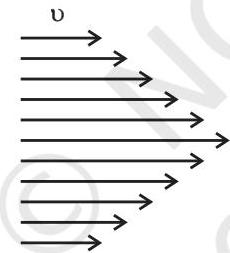 Fig. 9.13 Measurement of the coefficient of viscosity of a liquid.
The coefficient of viscosity, denoted by $\eta$ (pronounced 'eta'), for a fluid is formally defined as the quotient of the shearing stress divided by the strain rate.
$ \eta = \frac {F / A}{v / l} = \frac {F l}{v A} \tag {9.16} $
The standard international (SI) unit for viscosity is the poiseuille (Pl), though it is also commonly expressed in units of $\mathrm{N} , \mathrm{s} , \mathrm{m}^{-2}$ or $\mathrm{Pa} , \mathrm{s}$. The dimensional formula for viscosity is $[\mathrm{ML}^{-1} , \mathrm{T}^{-1}]$. Typically, fluids characterized as "thin," such as water and alcohol, exhibit lower viscosity compared to "thick" liquids, which include substances like coal tar, blood, and glycerine. The specific coefficients of viscosity for various common fluids are presented in Table 9.2. It is noteworthy to highlight two observations concerning blood and water. As demonstrated in Table 9.2, blood is notably more viscous, or 'thicker,' than water. Furthermore, the relative viscosity of blood, calculated as $(\eta / \eta_{\text{water}})$, maintains a consistent value across the temperature range of $0^{\circ} , \mathrm{C}$ to $37^{\circ} , \mathrm{C}$.
The intrinsic resistance to flow, or viscosity, in liquids typically diminishes as temperature rises, whereas for gases, this property generally exhibits an increase with elevated temperature.
Example 9.8 Consider a metallic block, possessing a surface area of $0.10\mathrm{m}^2$, linked to a $0.010\mathrm{kg}$ mass by means of a string routed over an idealized pulley (assumed to be devoid of mass and friction), as depicted in Figure 9.13. A fluid layer, $0.30\mathrm{mm}$ thick, is situated between the block and the underlying surface. Upon release, the block proceeds to move horizontally to the right at a constant velocity of $0.085\mathrm{ms}^{-1}$. Determine the dynamic viscosity coefficient of the intervening fluid.
Answer The metallic block's rightward motion is instigated by the tension within the connecting string. This tension, denoted $T$, is equivalent in magnitude to the gravitational force acting on the suspended mass $m$. Consequently, the shear force $F$ can be expressed as:
$ F = T = m g = 0.010 , \mathrm{kg} \times 9.8 , \mathrm{m} , \mathrm{s}^{-2} = 9.8 \times 10^{-2} , \mathrm{N} $
Shear stress on the fluid $= F / A = \frac{9.8 \times 10^{-2}}{0.10} , \mathrm{N/m}^2$
$ \text{Strain rate} = \frac{v}{l} = \frac{0.085}{0.30 \times 10^{-3}} , \mathrm{s}^{-1} $
$ \begin{array}{l} \eta = \frac{\text{stress}}{\text{strain rate}} \ = \frac{(9.8 \times 10^{-2} , \mathrm{N}) (0.30 \times 10^{-3} , \mathrm{m})}{(0.085 , \mathrm{m} , \mathrm{s}^{-1}) (0.10 , \mathrm{m}^2)} \ = 3.46 \times 10^{-3} , \mathrm{Pa} , \mathrm{s} \ \end{array} $
Table 9.2 presents the viscosities of selected fluid substances.
| Fluid | T(℃) | Viscosity (mP) |
|---|---|---|
| Water | 20 | 1.0 |
| 100 | 0.3 | |
| Blood | 37 | 2.7 |
| Machine Oil | 16 | 113 |
| 38 | 34 | |
| Glycerine | 20 | 830 |
| Honey | - | 200 |
| Air | 0 | 0.017 |
| 40 | 0.019 |
9.5.1 Stokes' Law
As an object traverses a fluid medium, it imparts motion to the adjacent fluid layer. This interaction generates relative movement between the various fluid strata, leading to the imposition of a resistive force on the object. Illustrative instances of this phenomenon include the descent of raindrops and the oscillation of pendulum bobs. Observations indicate that this viscous force is directly proportional to the object's velocity and acts in opposition to its trajectory. Furthermore, the magnitude of this force $F$ is influenced by the fluid's dynamic viscosity $\eta$ and the sphere's radius $a$. Sir George G. Stokes (1819-1903), a distinguished English scientist, precisely formulated this viscous drag force $F$ as
$ F = 6 \pi \eta a v \tag{9.17} $
This relation is recognized as Stokes' law. Its derivation will not be presented here.
Stokes' law provides a compelling illustration of a resistive force directly proportional to velocity. Let us examine its implications for an object descending through a viscous environment. Consider, for example, a raindrop in the atmosphere. Initially, it undergoes acceleration under the influence of gravity. As its speed escalates, the opposing resistive force concurrently intensifies. Eventually, a state of equilibrium is reached where the combined viscous and buoyant forces precisely counterbalance the gravitational force, resulting in a net force of zero and, consequently, zero acceleration. At this juncture, the spherical object (raindrop) continues its descent at a constant velocity. This constant velocity, termed the terminal velocity $\nu_{i}$, is thus expressed in equilibrium as
$ 6 \pi \eta a v_{i} = (4 \pi / 3) a^{3} (\rho - \sigma) g $
wherein $\rho$ denotes the mass density of the sphere and $\sigma$ represents the mass density of the fluid. Consequently, we derive
$ v_{i} = 2 a^{2} (\rho - \sigma) g / (9 \eta) \tag{9.18} $
Hence, the terminal velocity $\nu_{i}$ exhibits a dependence proportional to the square of the sphere's radius and inversely proportional to the viscosity of the surrounding medium.
You may like to refer back to Example 6.2 in this context.
Example 9.9 A copper sphere with a radius of $2.0 , \mathrm{mm}$ descends through an oil tank maintained at $20^{\circ} \mathrm{C}$, achieving a terminal velocity of $6.5 , \mathrm{cm} , \mathrm{s}^{-1}$. Calculate the dynamic viscosity of the oil at this temperature. The density of the oil is given as $1.5 \times 10^{3} , \mathrm{kg} , \mathrm{m}^{-3}$, and that of copper is $8.9 \times 10^{3} , \mathrm{kg} , \mathrm{m}^{-3}$.
Answer Given: $\nu_{i} = 6.5 \times 10^{-2} , \mathrm{ms}^{-1}$, $a = 2 \times 10^{-3} , \mathrm{m}$, $g = 9.8 , \mathrm{ms}^{-2}$, $\rho = 8.9 \times 10^{3} , \mathrm{kg} , \mathrm{m}^{-3}$
$ \sigma = 1.5 \times 10^{3} , \mathrm{kg} , \mathrm{m}^{-3}. \text{ From Eq. (9.18)} $
$ \begin{array}{l} \eta = \frac{2}{9} \times \frac{(2 \times 10^{-3})^{2} , \mathrm{m}^{2} \times 9.8 , \mathrm{m} , \mathrm{s}^{-2}}{6.5 \times 10^{-2} , \mathrm{m} , \mathrm{s}^{-1}} \times 7.4 \times 10^{3} , \mathrm{kg} , \mathrm{m}^{-3} \ = 9.9 \times 10^{-1} , \mathrm{kg} , \mathrm{m}^{-1} , \mathrm{s}^{-1} \ \end{array} $
9.6 SURFACE TENSION
Everyday observations reveal various intriguing phenomena: oil and water do not intermix; water adheres to human skin but not to a duck's plumage; mercury repels glass surfaces while water wets them; oil ascends a cotton wick against the pull of gravity. The ascent of sap and water to the uppermost foliage of trees; the bristles of a paintbrush, which remain separate when dry or immersed, coalesce into a fine point upon withdrawal from liquid. These phenomena, among numerous others, are intrinsically linked to the free interfaces of liquids. Since liquids possess a definite volume but lack a fixed shape, they naturally form a free surface when contained. These interfacial regions exhibit an inherent excess of energy. This characteristic behavior is termed surface tension, a property exclusive to liquids, as gases do not manifest distinct free surfaces. Let us now delve into the underlying principles of this phenomenon.
9.6.1 Surface Energy
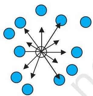
The cohesive integrity of a liquid is sustained by intermolecular attractive forces. Let us examine a molecule situated deep within the bulk of a liquid. Its spatial arrangement allows it to experience attractive interactions with all adjacent molecules [Fig. 9.14(a)]. Such interactions confer a negative potential energy upon the molecule, the magnitude of which is contingent upon the count and spatial arrangement of surrounding molecular entities. Nevertheless, the mean potential energy across all molecules within the bulk remains uniform. This assertion is substantiated by the substantial heat of evaporation required to disassociate a collection of these molecules (i.e., the liquid) into a gaseous state, separating them sufficiently. For instance, water necessitates an enthalpy of vaporization approximately $40\mathrm{kJ/mol}$.
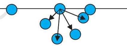
Now, consider a molecule positioned proximate to the liquid-vapor interface [Fig. 9.14(b)]. It is enveloped by liquid molecules solely on its inferior aspect. While it possesses a negative potential energy from these interactions, this energy is demonstrably less negative than that of a molecule entirely within the bulk phase. Its value is roughly half that of an interior molecule. Consequently, molecules residing at the liquid surface exhibit an elevated energy state relative to those in the bulk interior. Therefore, a liquid inherently seeks to minimize its surface area, constrained only by ambient conditions. Any expansion of the surface area necessitates an input of energy. The majority of surface phenomena can be elucidated through this fundamental principle. What is the energetic cost associated with situating a molecule at the surface? As previously noted, this energy approximates half the total energy required to completely liberate the molecule from the liquid phase, corresponding to half the heat of evaporation.
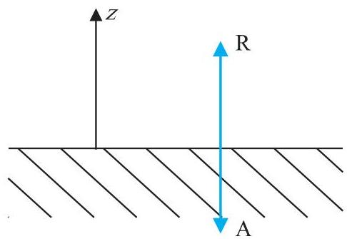
To conclude, how is a liquid surface precisely defined? Given the perpetual motion of constituent molecules within a liquid, the concept of a perfectly distinct or sharp interface is untenable. The molecular density of the liquid diminishes precipitously to zero in the vicinity of $z = 0$, spanning a distance equivalent to a few molecular dimensions, as depicted in Fig. 9.14(c).
 (a)
(a)
 (b)
(b)
 (c)
Fig. 9.14 Schematic picture of molecules in a liquid, at the surface and balance of forces. (a) Molecule inside a liquid. Forces on a molecule due to others are shown. Direction of arrows indicates attraction of repulsion. (b) Same, for a molecule at a surface. (c) Balance of attractive (AI and repulsive (R) forces.
(c)
Fig. 9.14 Schematic picture of molecules in a liquid, at the surface and balance of forces. (a) Molecule inside a liquid. Forces on a molecule due to others are shown. Direction of arrows indicates attraction of repulsion. (b) Same, for a molecule at a surface. (c) Balance of attractive (AI and repulsive (R) forces.
9.6.2 Surface Energy and Surface Tension
As previously established, an inherent excess energy is associated with the surface of liquids. Consequently, increasing the surface area (i.e., spreading the surface) while maintaining a constant volume necessitates an input of energy.
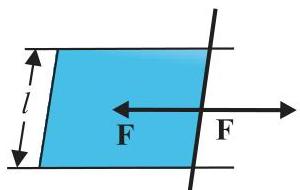
This phenomenon can be illustrated by considering a horizontal liquid film, which is bounded by parallel guides and terminates in a bar that is free to slide, as shown in Fig. 9.15.
 (a)
(a)
 (b)
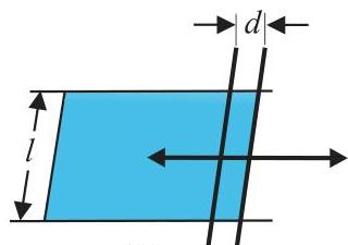
Fig. 9.15 Stretching a film. (a) A film in equilibrium; (b) The film stretched an extra distance.
(b)
Fig. 9.15 Stretching a film. (a) A film in equilibrium; (b) The film stretched an extra distance.
If we displace the bar by a small distance $d$, as depicted, the surface area increases. This increase in surface area implies that the system now possesses greater energy, indicating that work has been performed against an internal resistive force. Let this internal force be denoted by $\mathbf{F}$. The work done by the applied force is given by $\mathbf{F} \cdot \mathbf{d} = Fd$. According to the principle of energy conservation, this work is stored as additional energy within the liquid film. If $S$ represents the surface energy of the film per unit area, and considering that a film has two surfaces, the incremental area created is $2dl$. Thus, the additional energy stored is:
$ S (2 d l) = F d \tag {9.19} $
$ \operatorname {Or}, S = F d / 2 d l = F / 2 l \tag {9.20} $
This quantity, $S$, defines the magnitude of surface tension. It is equivalent to the surface energy per unit area of the liquid interface and also corresponds to the force per unit length exerted by the fluid on the movable bar.
Our discussion so far has focused on the surface of a single liquid. More broadly, it is essential to consider fluid surfaces that are in contact with other fluids or with solid surfaces. In such scenarios, the surface energy is contingent upon the properties of the materials on both sides of the interface. For instance, if the molecules of the contacting materials exhibit mutual attraction, the surface energy is reduced, whereas if they repel each other, the surface energy is increased. Therefore, it is more precise to consider surface energy as the energy associated with the interface between two materials, which is influenced by both materials.
From the foregoing analysis, we derive the following observations:
(i) Surface tension is defined as a force per unit length (or, alternatively, surface energy per unit area) acting within the plane of the interface between the liquid and any other substance. It also represents the surplus energy possessed by molecules at the interface compared to those situated in the bulk interior. (ii) At any point on the interface, excluding its physical boundaries, one can conceptualize a line. Along this line, equal and opposite surface tension forces, $S$ per unit length, act perpendicularly to the line within the plane of the interface, signifying that the line is in equilibrium. To elaborate, imagine a linear arrangement of atoms or molecules at the surface. The atoms to the left exert an attractive pull on this line, while those to the right exert a similar pull in their direction. This line of atoms is thus held in equilibrium under tension. However, if such a line truly delineates the boundary of the interface, as depicted in Figure 9.14 (a) and (b), then only an inward force of $S$ per unit length is observed.
Table 9.3 presents the surface tension values for several liquids. Surface tension is temperature-dependent; similar to viscosity, it typically decreases as the temperature rises.
Table 9.3: Surface Tension and Heats of Vaporization for Selected Liquids at Specified Temperatures
| Liquid | Temp(℃) | Surface Tension (N/m) | Heat of vaporisation (kJ/mol) |
|---|---|---|---|
| Helium | -270 | 0.000239 | 0.115 |
| Oxygen | -183 | 0.0132 | 7.1 |
| Ethanol | 20 | 0.0227 | 40.6 |
| Water | 20 | 0.0727 | 44.16 |
| Mercury | 20 | 0.4355 | 63.2 |
Adhesion of a fluid to a solid surface occurs when the interfacial energy between the fluid and the solid is less than the combined surface energies of the solid-air and fluid-air interfaces. This implies an attractive force between the solid surface and the liquid. An experimental setup for directly quantifying this phenomenon is depicted schematically in Fig. 9.16. In this arrangement, a flat, vertically oriented glass plate, positioned above a container holding a liquid, constitutes one side of a balance apparatus. The plate is counterbalanced by weights on the opposing side, with its lower horizontal edge situated just above the liquid's surface. The liquid container is then gently elevated until the liquid makes contact with the glass plate, at which point the surface tension exerts a downward pull on the plate. Additional weights are subsequently applied until the plate separates from the liquid surface.
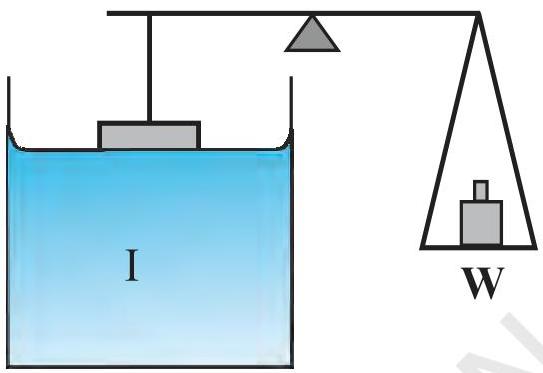 Fig. 9.16 Measuring Surface Tension.
Assuming the supplementary weight necessary is $W$ . Then, referencing Equation 9.20 and its accompanying explanation, the surface tension at the liquid-air interface can be expressed as:
$ S _ {\mathrm {l a}} = (W / 2 l) = (m g / 2 l) \tag {9.21} $
Here, $m$ signifies the incremental mass, and $l$ denotes the length of the plate's edge. The subscript (la) serves to underscore that the tension at the liquid-air boundary is the quantity being considered.
9.6.3 Angle of Contact
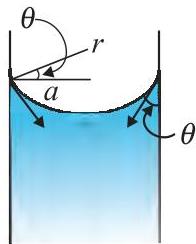
The surface of a liquid, when in proximity to a different medium at its plane of contact, generally exhibits curvature. The angle of contact is defined as the angle formed between the tangent to the liquid's surface at the precise point of contact and the solid surface, measured from within the liquid phase. This angle is represented by $\theta$. Its value is distinct for various combinations of liquids and solids at their interfaces. The magnitude of $\theta$ is crucial in determining whether a liquid will spread across a solid surface or instead coalesce into individual droplets upon it. For instance, water forms droplets on a lotus leaf, as depicted in Fig. 9.17 (a), while it spreads extensively over a clean plastic plate, as illustrated in Fig. 9.17(b).
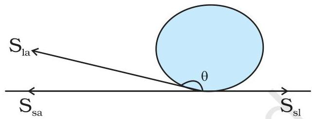
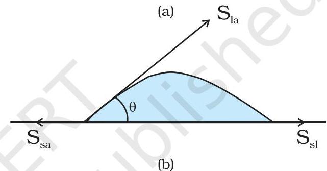 Fig. 9.17 Different shapes of water drops with interfacial tensions (a) on a lotus leaf (b) on a clean plastic plate.
We consider the three interfacial tensions present at the three distinct interfaces—liquid-air, solid-air, and solid-liquid—which are designated as $S_{\mathrm{la}}$, $S_{\mathrm{sa}}$, and $S_{\mathrm{sl}}$, respectively, as referenced in Fig. 9.17 (a) and (b). Along the line where these three media meet, the surface forces must be in a state of equilibrium. From Fig. 9.17(b), the following relationship can be readily derived:
$ S _ {\mathrm {l a}} \cos \theta + S _ {\mathrm {s l}} = S _ {\mathrm {s a}} \tag {9.22} $
The angle of contact is an obtuse angle if $S_{\mathrm{sl}} > S_{\mathrm{la}}$, as observed in the case of a water-leaf interface. Conversely, it is an acute angle when $S_{\mathrm{sl}} < S_{\mathrm{la}}$, exemplified by the water-plastic interface. When $\theta$ is an obtuse angle, it signifies that the liquid molecules are strongly attracted to each other (cohesive forces) but weakly attracted to the solid molecules (adhesive forces). Consequently, a substantial amount of energy is expended to create a liquid-solid surface, preventing the liquid from wetting the solid. This phenomenon is evident with water on waxy or oily surfaces, and similarly, with mercury on
any solid surface. Conversely, should the liquid molecules possess a strong affinity for the solid's molecules, this interaction effectively lowers $S_{\mathrm{sl}}$. This reduction, in turn, can lead to an increase in $\cos \theta$ or a decrease in $\theta$, resulting in an acute angle. This behavior characterizes water on glass or plastic, and kerosene oil, which readily spreads on most materials. Substances such as soaps, detergents, and dyeing agents function as wetting agents; their inclusion diminishes the angle of contact, thereby enhancing penetration and efficacy. In contrast, waterproofing agents are designed to increase the angle of contact between water and textile fibers.
9.6.4 Drops and Bubbles
The phenomenon of surface tension dictates that isolated liquid droplets and bubbles assume a spherical geometry, provided gravitational influences are negligible. This characteristic is often vividly observed in minute droplets emanating from high-velocity sprays or jets, as well as in the familiar soap bubbles created during recreational activities. This raises fundamental questions: What mechanism compels drops and bubbles to adopt a spherical form? Furthermore, what factors contribute to the stability of soap bubbles?
As previously established, any interface between a liquid and air possesses inherent energy. Consequently, for a fixed volume, the configuration that minimizes this energy corresponds to the surface exhibiting the smallest possible area. The spherical shape uniquely satisfies this criterion. While a detailed mathematical derivation falls outside the purview of this text, it can be demonstrated that a sphere is geometrically superior to other forms, such as a cube, in terms of minimizing surface area for a given volume. Therefore, in the absence of gravitational forces and other external influences like air resistance, liquid droplets would naturally assume a perfectly spherical shape.
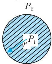
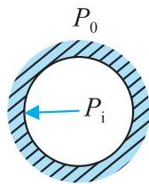
A further noteworthy implication of surface tension is that the internal pressure within a spherical droplet (illustrated in Fig. 9.18(a)) exceeds the external pressure. Consider a spherical droplet of radius $r$ maintained in equilibrium. Should its radius undergo an incremental expansion of $\Delta r$, the resultant increase in surface energy is given by:
$ [4\pi(r + \Delta r)^2 - 4\pi r^2] S_{\mathrm{la}} = 8\pi r \Delta r S_{\mathrm{la}} \tag{9.23} $
In a state of equilibrium, this energetic expenditure is precisely counteracted by the energetic gain derived from the expansion against the pressure differential $(P_{\mathrm{i}} - P_{0})$ existing between the droplet's interior and its exterior. The work performed during this expansion is:
$ W = (P_{\mathrm{i}} - P_{0}) 4\pi r^2 \Delta r \tag{9.24} $
leading to the relation:
$ (P_{\mathrm{i}} - P_{0}) = (2 S_{\mathrm{la}} / r) \tag{9.25} $
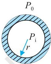
More broadly, across any liquid-gas interface, the pressure on the convex surface invariably surpasses that on the concave surface. Illustratively, an air bubble suspended within a liquid will experience a higher internal pressure. Refer to Fig. 9.18 (b).
 (a)
(a)
 (b)
(b)
 (c)
Fig. 9.18 Drop, cavity and bubble of radius $r$.
(c)
Fig. 9.18 Drop, cavity and bubble of radius $r$.
A bubble, as depicted in Fig. 9.18 (c), is distinct from both a liquid drop and a cavity, fundamentally due to its possession of two distinct liquid-air interfaces. Extending the preceding derivation to the case of a bubble yields:
$ (P_{\mathrm{i}} - P_{0}) = (4 S_{\mathrm{la}} / r) \tag{9.26} $
This physical principle elucidates why a certain degree of effort, yet not excessive force, is requisite to inflate a soap bubble. A modest elevation in internal air pressure is essential for its formation!
9.6.5 Capillary Rise
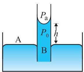
A notable outcome of the pressure differential existing across a curved liquid-air boundary is the familiar phenomenon of liquid ascending within a narrow tube, even against gravitational forces. The term "capilla" originates from Latin, meaning hair; indeed, if the tube possessed hair-like fineness, the observed rise would be substantial. To elucidate this, consider a vertical capillary tube of circular cross-section (with radius 'a') inserted into an open container of water (Fig. 9.19). The contact angle between water and
 (a)
(a)
 (b)
Fig. 9.19 Capillary rise, (a) Schematic picture of a narrow tube immersed water. (b) Enlarged picture near interface.
(b)
Fig. 9.19 Capillary rise, (a) Schematic picture of a narrow tube immersed water. (b) Enlarged picture near interface.
glass is acute. Consequently, the water surface within the capillary tube forms a concave meniscus. This configuration implies a pressure difference across the two sides of this upper liquid surface, which is expressed by:
$ \begin{array}{l} (P_{l} - P_{0}) = (2S/r) = 2S/(a \sec \theta) \ = (2S/a) \cos \theta \tag{9.27} \end{array} $
Thus, the pressure of the water inside the tube, precisely at the meniscus (the air-water interface), registers as less than the ambient atmospheric pressure. Consider the two points A and B as depicted in Fig. 9.19(a). These points must necessarily be at an equivalent pressure, specifically:
$ P_{0} + h \rho g = P_{l} = P_{A} \tag{9.28} $
where $\rho$ denotes the density of water and $h$ is termed the capillary rise [Fig. 9.19(a)]. By utilizing Equations (9.27) and (9.28), we derive:
$ h \rho g = (P_{l} - P_{0}) = (2S \cos \theta)/a \tag{9.29} $
The foregoing discussion, in conjunction with Eqs. (9.24) and (9.25), unequivocally establishes that capillary ascent is attributable to surface tension. Its magnitude increases with a reduction in 'a'. Typically, for fine capillaries, this rise is on the order of a few centimeters. For example, if $a = 0.05$ cm, employing the surface tension value for water (from Table 9.3) yields:
$ \begin{array}{l} h = 2S/(\rho g a) \ = \frac{2 \times (0.073 \ \mathrm{N \ m^{-1}})}{(10^{3} \ \mathrm{kg \ m^{-3}}) \ (9.8 \ \mathrm{m \ s^{-2}})(5 \times 10^{-4} \ \mathrm{m})} \ = 2.98 \times 10^{-2} \ \mathrm{m} = 2.98 \ \mathrm{cm} \end{array} $
It is important to note that if the liquid meniscus exhibits a convex curvature, as observed with mercury, i.e., if $\cos \theta$ is negative, then, as can be deduced from Eq. (9.28) for instance, the liquid level will clearly be depressed within the capillary!
Example 9.10 The lower end of a capillary tube of diameter $2.00 \ \mathrm{mm}$ is dipped 8.00 cm below the surface of water in a beaker. What is the pressure required in the tube in order to blow a hemispherical bubble at its end in water? The surface tension of water at temperature of the experiments is $7.30 \times 10^{-2} \ \mathrm{Nm^{-1}}$. 1 atmospheric pressure = $1.01 \times 10^{5} \ \mathrm{Pa}$, density of water = $1000 \ \mathrm{kg/m^3}$, $g = 9.80 \ \mathrm{m \ s^{-2}}$. Also calculate the excess pressure.
Answer The overpressure within a gas bubble submerged in a liquid is quantified by the expression $2S/r$, where $S$ represents the surface tension at the liquid-gas interface. It is crucial to recognize that in this specific scenario, only a single liquid surface is involved. (Conversely, for a liquid bubble encapsulated within a gas, two liquid surfaces are present, necessitating the use of $4S/r$ for the excess pressure calculation.) The variable $r$ denotes the bubble's radius. Consequently, the external pressure $P_{0}$ acting on the bubble equates to the sum of the atmospheric pressure and the hydrostatic pressure exerted by an $8.00 \ \mathrm{cm}$ column of water. This can be stated as:
$ \begin{array}{l} P_{0} = (1.01 \times 10^{5} \ \mathrm{Pa} + 0.08 \ \mathrm{m} \times 1000 \ \mathrm{kg \ m^{-3}} \ \quad \times 9.80 \ \mathrm{m \ s^{-2}}) \ = 1.01784 \times 10^{5} \ \mathrm{Pa} \end{array} $
Therefore, the pressure inside the bubble is
$ \begin{array}{l} P_{l} = P_{0} + 2S/r \ = 1.01784 \times 10^{5} \ \mathrm{Pa} + (2 \times 7.3 \times 10^{-2} \ \mathrm{Pa \ m/10^{-3} \ m}) \ = (1.01784 + 0.00146) \times 10^{5} \ \mathrm{Pa} \ = 1.02 \times 10^{5} \ \mathrm{Pa} \end{array} $
The radius of the bubble is considered equivalent to that of the capillary tube, a premise supported by its hemispherical geometry. It is important to note that the final numerical result has been approximated to three significant figures. Consequently, the surplus pressure within the bubble amounts to $146 \ \mathrm{Pa}$.
SUMMARY
- A fundamental characteristic of a fluid is its capacity for flow. Fluids inherently lack resistance to alterations in their form. Consequently, a fluid's configuration is dictated by the vessel containing it.
- Liquids are characterized by their incompressibility and the presence of a distinct free surface. Conversely, gases exhibit compressibility and will expand to completely fill any volume accessible to them.
- Should $F$ represent the normal force exerted by a fluid upon an area $A$, then the average pressure, $P_{av}$, is formally defined as the quotient of this force and the area:
$ P_{av} = \frac{F}{A} $
The standard unit for pressure is the pascal (Pa), which is dimensionally equivalent to N m⁻². Additional frequently encountered units of pressure include: 1 atm = 1.01 × 10⁵ Pa 1 bar = 10⁵ Pa 1 torr = 133 Pa = 0.133 kPa 1 mm of Hg = 1 torr = 133 Pa
Pascal's law postulates that within a static fluid, the pressure is uniform across all points situated at an identical elevation. Furthermore, any alteration in pressure applied to a confined fluid is propagated without reduction throughout every portion of the fluid and to the boundaries of its containment.
The pressure within a fluid exhibits variation with depth $h$, as described by the relation:
$ P = P₀ + ρgh $
In this equation, ρ denotes the fluid's density, which is presumed to be uniform.
- For an incompressible fluid undergoing steady flow within a pipe of varying cross-sectional area, the volumetric flow rate, or the volume passing any given point per unit time, remains invariant.
$ vA = \text {constant} $
(where v represents velocity and A denotes the cross-sectional area) This relationship is a direct consequence of the principle of mass conservation applied to incompressible fluid dynamics.
- Bernoulli's principle asserts that along a streamline, the aggregate of the pressure (P), the kinetic energy per unit volume (ρv²/2), and the potential energy per unit volume (ρgy) maintains a constant value.
$ P + ρv²/2 + ρgy = \text {constant} $
This equation fundamentally represents the application of energy conservation to the steady-state motion of an inviscid fluid. Given that no fluid possesses absolutely zero viscosity, the aforementioned statement holds true only as an approximation. Viscosity acts analogously to friction, transducing kinetic energy into thermal energy.
- While a fluid does not necessitate the presence of shear stress to exhibit shear strain, the application of shear stress to a fluid instigates motion, leading to a time-dependent increase in shear strain. The coefficient of viscosity, η, is defined as the ratio of the shear stress to the temporal rate of shearing strain,
$ \eta = \frac{\text{Shear stress}}{\text{Rate of shear strain}} $
where all symbols carry their conventional interpretations and are explicated within the accompanying text.
Stokes' law defines the viscous resistance force (F) experienced by a spherical object of radius 'a' traveling at velocity 'v' through a fluid with dynamic viscosity 'η' as, F = 6πηav.
Surface tension is characterized as a force per unit length (alternatively, surface energy per unit area) exerted within the interfacial plane separating a liquid from its confining boundary. This phenomenon stems from the elevated energy state of molecules situated at the interface compared to those within the bulk of the liquid.
POINTS TO PONDER
Pressure is fundamentally a scalar magnitude. Although its definition as "force per unit area" might misleadingly suggest a vector quantity, the force component referenced in this definition is exclusively that which acts perpendicularly to the surface it impinges upon. When conceptualizing fluids, it becomes necessary to transition away from the paradigms of particle and rigid body mechanics, focusing instead on characteristics that exhibit spatial variation throughout the fluid medium.
It is incorrect to conceive of fluid pressure as being exerted solely upon solid boundaries, such as container walls or submerged solid objects. Rather, pressure is present ubiquitously throughout a fluid. A fluid element (for instance, as depicted in Fig. 9.4) maintains equilibrium due to the equivalence of pressures acting upon its diverse surfaces.
The pressure expression,
$ P = P_{s} + \rho gh $
is accurate when the fluid is incompressible. From a practical standpoint, this applies to liquids, which are largely incompressible, meaning their density remains nearly constant with height.
- Gauge pressure is defined as the disparity between the absolute pressure and the ambient atmospheric pressure, expressed as
$ P - P_{s} = P_{g} $
Numerous instruments designed for pressure measurement, such as tire pressure gauges and sphygmomanometers (blood pressure monitors), directly indicate gauge pressure.
A streamline serves as a graphical representation of fluid flow. In a steady flow regime, two distinct streamlines cannot intersect; such an intersection would imply that a fluid particle possesses two simultaneous velocities at a single location, which is physically impossible.
Bernoulli's principle is inapplicable when viscous drag forces act upon the fluid. In such scenarios, the energy dissipated by these viscous forces must be integrated into the analysis, resulting in a pressure $P_{2}$ [Fig. 9.9] that is diminished relative to the value predicted by Eq. (9.12).
With an increase in temperature, liquid atoms exhibit heightened mobility, leading to a reduction in the coefficient of viscosity, $\eta$. Conversely, for gases, an elevation in temperature intensifies the random movement of atoms, which in turn causes $\eta$ to increase.
Surface tension originates from the surplus potential energy possessed by molecules at a surface, relative to the potential energy of molecules within the bulk of the material. This interfacial energy manifests at the boundary between any two substances, provided at least one of them is a fluid. Consequently, it is not an intrinsic characteristic of a solitary fluid.
| Physical Quantity | Symbol | Dimensions | Unit | Remarks |
|---|---|---|---|---|
| Pressure | P | [M L^{-1}T^{-2}] | pascal (Pa) | 1 atm = 1,013 × 10^{5} Pa, Scalar |
| Density | ρ | [M L^{-3}] | kg m^{-3} | Scalar |
| Specific Gravity | No | No | Ratio of substance density to water density; Scalar | |
| Co-efficient of viscosity | η | [M L^{-1}T^{-1}] | Pa s or Poiseuille (Pl) | Scalar |
| Surface Tension | S | [M T^{-2}] | N m^{-1} | Scalar |
EXERCISES
9.1 Explain why
(a) Human blood pressure exhibits higher values in the lower extremities compared to the cerebral region. (b) The atmospheric pressure observed at an altitude of approximately $6\mathrm{km}$ is reduced to nearly fifty percent of its sea-level magnitude, notwithstanding that the total extent of the atmosphere surpasses $100\mathrm{km}$. (c) Hydrostatic pressure is classified as a scalar magnitude, despite the fact that pressure itself is defined as the ratio of force to area.
9.2 Explain why
(a) The contact angle formed by mercury on a glass surface is obtuse, whereas that formed by water on glass is acute. (b) When introduced to a pristine glass surface, water typically exhibits a tendency to spread, whereas mercury on an identical surface tends to coalesce into discrete droplets. (Alternatively stated, water demonstrates wetting behavior on glass, while mercury does not.)
(c) The surface tension exhibited by a liquid does not vary with the superficial area it occupies. (d) Aqueous solutions containing dissolved detergent ought to display diminutive contact angles. (e) In the absence of external forces, a liquid droplet invariably assumes a spherical morphology.
9.3 Fill in the blanks using the word(s) from the list appended with each statement:
(a) The surface tension of liquids typically ... with rising temperatures (increases / decreases) (b) The viscosity of gases generally ... as temperature rises, while the viscosity of liquids ... with temperature (increases / decreases) (c) In solids possessing an elastic modulus of rigidity, the shearing force is directly proportional to ... , whereas for fluids, it is proportional to ... (shear strain / rate of shear strain) (d) For a fluid exhibiting steady flow, the augmentation in flow velocity within a constricted region adheres to (conservation of mass / Bernoulli's principle) (e) In the context of an aircraft model within a wind tunnel, turbulent flow manifests at a ... velocity compared to the onset of turbulence for a full-scale aircraft (greater / smaller)
9.4 Explain why
(a) To maintain a sheet of paper in a horizontal orientation, one should direct an airstream above it, rather than beneath it. (b) Attempting to obstruct a water faucet with one's fingers results in rapid streams of water forcefully ejecting through the interstices between the digits. (c) The bore diameter of a hypodermic needle exerts a more significant influence on the flow rate than the manual pressure applied by a physician during the administration of an injection. (d) The efflux of a fluid from a small aperture in a container generates a reactive thrust upon the container itself. (e) An airborne, rotating cricket ball deviates from a purely parabolic flight path.
9.5 A female individual weighing $50 \mathrm{kg}$, attired in high-heeled footwear, maintains equilibrium on one heel. This heel possesses a circular cross-section with a diameter of $1.0 \mathrm{cm}$. Calculate the pressure exerted by this heel upon a horizontal surface.
9.6 Torricelli's barometer employed mercury. Pascal replicated this experiment utilizing French wine, which has a density of $984 \mathrm{kg} \mathrm{m}^{-3}$. Ascertain the requisite height of the wine column to balance standard atmospheric pressure.
9.7 An upright offshore installation is engineered to tolerate a peak stress of $10^9 \mathrm{Pa}$. Would this construction be appropriate for deployment above an oceanic oil well? Assume an approximate ocean depth of $3 \mathrm{km}$, and disregard the influence of ocean currents.
9.8 A hydraulic vehicle hoist is configured to elevate automobiles with a peak mass of $3000 \mathrm{kg}$. The cross-sectional area of the piston supporting the load measures $425 \mathrm{cm}^2$. What is the maximum pressure that the smaller piston would be required to sustain?
9.9 Within a U-shaped tube, water and methylated spirit are demarcated by mercury. The mercury levels in both limbs are coincident, with $10.0 \mathrm{cm}$ of water occupying one limb and $12.5 \mathrm{cm}$ of spirit occupying the other. Determine the specific gravity of the spirit.
9.10 Referring to the preceding problem, should an additional $15.0 \mathrm{cm}$ of both water and spirit be introduced into their respective arms of the tube, what would be the resulting disparity in the mercury levels between the two arms? (Specific gravity of mercury = $13.6$)
9.11 Is Bernoulli's principle applicable for characterizing the movement of water through a river rapid? Provide an explanation.
9.12 Is there a material difference when employing gauge pressures versus absolute pressures in the application of Bernoulli's equation? Elucidate.
9.13 Glycerine traverses uniformly through a horizontal conduit of $1.5 \mathrm{m}$ length and $1.0 \mathrm{cm}$ radius. Given that the mass of glycerine accumulated per second at one extremity is $4.0 \times 10^{-3} \mathrm{kg} \mathrm{s}^{-1}$, what is the pressure differential across the two termini of the tube? (The density of glycerine is $1.3 \times 10^3 \mathrm{kg} \mathrm{m}^{-3}$, and its viscosity is $0.83 \mathrm{Pa} \mathrm{s}$). [It is also advisable to verify the validity of the laminar flow assumption within the tube].
9.14 During an experimental evaluation of an aircraft model within a wind tunnel, the fluid velocities over the superior and inferior surfaces of the aerofoil are recorded as $70 \mathrm{m} \mathrm{s}^{-1}$ and $63 \mathrm{m} \mathrm{s}^{-1}$, respectively. Determine the aerodynamic lift generated by the wing, given its surface area is $2.5 \mathrm{m}^2$. Assume the density of air to be $1.3 \mathrm{kg} \mathrm{m}^{-3}$.
9.15 Illustrations $9.20(\mathrm{a})$ and $(\mathrm{b})$ depict the uniform flow of an ideal (non-viscous) fluid. Identify which of these two illustrations is erroneous, and provide justification.
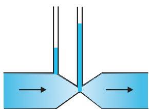 (a)
(a)
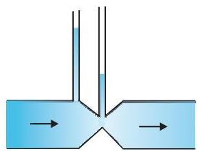 (b)
Fig. 9.20
(b)
Fig. 9.20
9.16 A spray pump features a cylindrical tube with a cross-sectional area of $8.0\mathrm{cm}^2$. At one extremity, there are 40 minute apertures, each measuring $1.0\mathrm{mm}$ in diameter. Given that the fluid's volumetric flow rate within the tube is $1.5\mathrm{mmin}^{-1}$, determine the velocity at which the liquid exits through these apertures.
9.17 Consider a U-shaped wire, immersed in a soap solution and subsequently withdrawn. The delicate soap film that forms between this wire and a lightweight slider is capable of sustaining a total load of $1.5 \times 10^{-2} \mathrm{N}$ (this value encompasses the minor mass of the slider itself). If the slider's length is $30 \mathrm{cm}$, calculate the surface tension exhibited by this film.
9.18 As depicted in Figure 9.21 (a), a slender liquid film is shown bearing a modest load of $4.5 \times 10^{-2} \mathrm{~N}$. Determine the magnitude of the load that would be sustained by a film of identical liquid, maintained at the same temperature, as illustrated in Fig. (b) and (c). Provide a physical explanation for your conclusion.
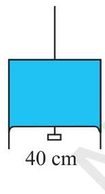 (a)
Fig. 9.21
(a)
Fig. 9.21
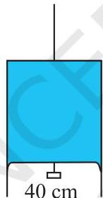 (b)
(b)
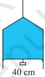 (c)
(c)
9.19 Calculate the internal pressure within a mercury droplet having a radius of $3.00\mathrm{mm}$ when at ambient temperature. The surface tension of mercury at this specific temperature $(20^{\circ}\mathrm{C})$ is reported as $4.65\times 10^{-1}\mathrm{Nm}^{-1}$. Given that the prevailing atmospheric pressure is $1.01\times 10^{5}\mathrm{Pa}$, also state the differential pressure (excess pressure) observed within the droplet. 9.20 Determine the surplus pressure within a spherical soap solution bubble of $5.00\mathrm{mm}$ radius, considering that the surface tension of the soap solution at a temperature of $(20^{\circ}\mathrm{C})$ is $2.50\times 10^{-2}\mathrm{Nm}^{-1}$. Furthermore, if an air bubble of identical size were to form at a depth of $40.0\mathrm{cm}$ within a vessel holding the same soap solution (which possesses a relative density of 1.20), what would be the absolute pressure inside this bubble? (Assume a standard atmospheric pressure of $1.01\times 10^{5}\mathrm{Pa}$).