CHAPTER TWO
MOTION IN A STRAIGHT LINE
2.1 Introduction
2.2 Instantaneous velocity and speed
2.3 Acceleration
2.4 Kinematic equations for uniformly accelerated motion
2.5 Relative velocity
Summary
Points to ponder
Exercises
2.1 INTRODUCTION
Motion is an inherent characteristic throughout the cosmos. We engage in activities such as walking, running, and cycling. Even during sleep, air continuously enters and exits our lungs, and blood circulates through arteries and veins. We observe phenomena like leaves detaching from trees and water cascading from a dam. Automobiles and aircraft facilitate human transport between locations. Earth completes one rotation every twenty-four hours and orbits the sun annually. The sun itself is in motion within the Milky Way galaxy, which, in turn, is traversing within its local galactic cluster.
Motion is defined as an object's change in spatial position over time. How does this position evolve with time? This chapter aims to elucidate methods for describing motion. To achieve this, we will develop the fundamental concepts of velocity and acceleration. Our discussion will be limited to the study of objects moving along a straight path, commonly known as rectilinear motion. For instances of rectilinear motion exhibiting constant acceleration, a straightforward set of equations can be derived. Finally, to grasp the relational aspect of motion, the concept of relative velocity will be introduced.
Throughout our discussions, objects in motion will be approximated as point objects. This simplification holds true when an object's physical dimensions are significantly smaller than the distance it covers within a considerable timeframe. In numerous real-world scenarios, the physical size of objects can be disregarded, allowing them to be treated as point-like entities with minimal analytical error.
Kinematics focuses on describing motion without exploring its underlying causes. The principles governing the causes of motion, which are distinct from the descriptions presented in this and the subsequent chapter, constitute the subject matter of Chapter 4.
2.2 INSTANTANEOUS VELOCITY AND SPEED
The concept of average velocity informs us about an object's overall rate of movement across a specific duration, yet it fails to convey its precise speed at various moments within that period. To address this limitation, we introduce the notion of instantaneous velocity, often referred to simply as velocity, denoted by $v$, at a particular moment $t$.
At any given instant, velocity is formally defined as the limiting value of the average velocity as the time interval, $\Delta t$, approaches an infinitesimal duration. Expressed mathematically:
$ v = \lim_{\Delta t \to 0} \frac{\Delta x}{\Delta t} \tag{2.1a} $
$ = \frac{\mathrm{d} x}{\mathrm{d} t} \tag{2.1b} $
Here, the notation $\frac{\lim}{\Delta t \to 0}$ represents the mathematical operation of determining the limit of the subsequent expression as $\Delta t$ tends towards zero. Within the framework of calculus, the term on the right-hand side of Eq. (2.1a) corresponds to the differential coefficient of $x$ concerning $t$, commonly symbolized as $\frac{\mathrm{d}x}{\mathrm{d}t}$ (refer to Appendix 2.1). Fundamentally, this signifies the instantaneous rate at which position changes with respect to time.
Equation (2.1a) offers a means to ascertain the instantaneous velocity at a particular moment, either through graphical interpretation or numerical computation. Consider, for instance, the objective of graphically determining the velocity at $t = 4 , \text{s}$ (designated as point P) for the car's movement depicted in Fig. 2.1. If we select a time interval $\Delta t = 2 , \text{s}$, symmetrically centered at $t = 4 , \text{s}$, then, consistent with the definition of average velocity, the gradient of the line segment $\mathrm{P}_1\mathrm{P}_2$ (as illustrated in Fig. 2.1) yields the average velocity spanning the interval from 3 s to 5 s.
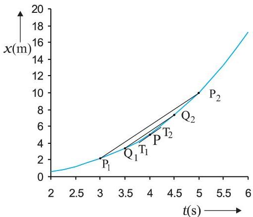 Fig. 2.1 Ascertaining velocity from a position-time plot. The velocity at $t = 4 , \text{s}$ corresponds to the gradient of the tangent line to the curve at that specific point in time.
Subsequently, if we reduce the magnitude of $\Delta t$ from 2 s to 1 s, the line segment $\mathrm{P}_1\mathrm{P}_2$ transforms into $\mathrm{Q}_1\mathrm{Q}_2$. Its gradient then represents the average velocity over the interval spanning 3.5 s to 4.5 s. As $\Delta t$ approaches zero, i.e., in the limit $\Delta t \to 0$, the line $\mathrm{P}_1\mathrm{P}_2$ converges to become the tangent to the position-time curve at point P. Consequently, the velocity at $t = 4 , \text{s}$ is precisely the slope of this tangent line at that specific point. While illustrating this dynamic graphically poses challenges, employing a numerical methodology to derive the velocity value effectively elucidates the concept of the limiting process. For the trajectory depicted in Fig. 2.1, the position is given by $x = 0.08 , t^3$. Table 2.1 presents the computed values of $\Delta x / \Delta t$ for various $\Delta t$ values—specifically 2.0 s, 1.0 s, 0.5 s, 0.1 s, and 0.01 s—each centered at $t = 4.0 , \text{s}$. The second and third columns list the values for $t_1 = \left(t - \frac{\Delta t}{2}\right)$ and $t_2 = \left(t + \frac{\Delta t}{2}\right)$, respectively, while the fourth and fifth columns present the corresponding position values, $x(t_1)$ and $x(t_2)$.
Table 2.1 Values of $\frac{\Delta x}{\Delta t}$ as $\Delta t$ diminishes, centered at $t = 4 , \text{s}$
| Δt(s) | t1(s) | t2(s) | x(t1)(m) | x(t2)(m) | Δx(m) | Δx / Δt(m·s-1) |
|---|---|---|---|---|---|---|
| 2.0 | 3.0 | 5.0 | 2.16 | 10.0 | 7.84 | 3.92 |
| 1.0 | 3.5 | 4.5 | 3.43 | 7.29 | 3.86 | 3.86 |
| 0.5 | 3.75 | 4.25 | 4.21875 | 6.14125 | 1.9225 | 3.845 |
| 0.1 | 3.95 | 4.05 | 4.93039 | 5.31441 | 0.38402 | 3.8402 |
| 0.01 | 3.995 | 4.005 | 5.100824 | 5.139224 | 0.0384 | 3.8400 |
MOTION IN A STRAIGHT LINE
The corresponding values of $x$, denoted as $x(t_1) = 0.08 t_1^3$ and $x(t_2) = 0.08 t_2^3$, are determined. The sixth column itemizes the displacement $\Delta x = x(t_2) - x(t_1)$, while the final column presents the quotient of $\Delta x$ and $\Delta t$, which signifies the average velocity associated with the $\Delta t$ value specified in the initial column.
Table 2.1 illustrates that a reduction in $\Delta t$ from $2.0,\mathrm{s}$ to $0.010,\mathrm{s}$ causes the average velocity to converge towards a limiting value of $3.84,\mathrm{ms}^{-1}$. This specific value represents the instantaneous velocity at $t = 4.0,\mathrm{s}$, precisely $\frac{dx}{dt}$ evaluated at that time point. This methodology allows for the determination of the car's velocity at any given instant.
Determining instantaneous velocity through graphical means is frequently impractical. Such an approach necessitates meticulous plotting of the position-time graph and the subsequent computation of average velocity as $\Delta t$ progressively diminishes. A more straightforward approach to ascertain velocity at various instants involves either possessing position data at discrete times or an explicit functional relationship for position with respect to time. In such cases, one can compute $\Delta x / \Delta t$ from the available data as $\Delta t$ decreases to derive the limiting value, as demonstrated in Table 2.1, or alternatively, employ differential calculus on the given expression to determine $\frac{dx}{dt}$ at specific moments, as illustrated in the subsequent example.
Example 2.1 An object's position along the $x$-axis is described by the equation $x = a + bt^2$, where $a = 8.5,\mathrm{m}$, $b = 2.5,\mathrm{ms}^{-2}$, and $t$ is expressed in seconds. Determine its velocity at $t = 0,\mathrm{s}$ and $t = 2.0,\mathrm{s}$. Calculate the average velocity between $t = 2.0,\mathrm{s}$ and $t = 4.0,\mathrm{s}$?
Answer Within the framework of differential calculus, the instantaneous velocity is expressed as:
$ v = \frac{dx}{dt} = \frac{d}{dt} \left(a + bt^2\right) = 2b t = 5.0 t m \mathrm{s}^{-1} $
Consequently, at $t = 0,\mathrm{s}$, the velocity is $v = 0,\mathrm{ms}^{-1}$, and at $t = 2.0,\mathrm{s}$, it is $v = 10,\mathrm{ms}^{-1}$.
$ \text{Average velocity} = \frac{x(4.0) - x(2.0)}{4.0 - 2.0} $
$ \begin{array}{l} = \frac{a + 16b - a - 4b}{2.0} = 6.0 \times b \ = 6.0 \times 2.5 = 15,\mathrm{ms}^{-1} \end{array} $
It is important to note that in uniform motion, the instantaneous velocity is consistently equivalent to the average velocity across all time intervals.
Instantaneous speed, often referred to simply as speed, is defined as the scalar magnitude of velocity. For instance, both a velocity of $+24.0,\mathrm{ms}^{-1}$ and a velocity of $-24.0,\mathrm{ms}^{-1}$ correspond to an identical speed of $24.0,\mathrm{ms}^{-1}$. It is pertinent to observe that while average speed across a finite duration is either greater than or equal to the magnitude of the average velocity, the instantaneous speed at any given moment is precisely equivalent to the magnitude of the instantaneous velocity at that specific moment. What accounts for this distinction?
2.3 ACCELERATION
The velocity of a moving object typically undergoes variation throughout its trajectory. A fundamental question arises regarding the appropriate method for quantifying this alteration: should it be characterized by the rate at which velocity changes with respect to distance, or with respect to time? This conceptual challenge was evident as early as Galileo's era. Initially, the prevailing thought posited that this alteration should be described by the rate of velocity change over distance. Nevertheless, Galileo's comprehensive investigations into the kinematics of freely falling bodies and objects traversing inclined planes led him to the pivotal conclusion that, for all objects in free fall, the rate of change of velocity with respect to time is a constant parameter of motion. In contrast, he observed that the change in velocity with respect to distance exhibits variability, specifically decreasing as the distance of descent increases. This critical insight ultimately paved the way for the development of the concept of acceleration, formally defined as the temporal rate of change of velocity.
Average acceleration, denoted as $\overline{a}$, is formally defined over a specific time interval as the quotient of the change in velocity and the duration of that interval:
$ \overline{a} = \frac{v_2 - v_1}{t_2 - t_1} = \frac{\Delta v}{\Delta t} \tag{2.2} $
Here, $v_1$ and $v_2$ represent the instantaneous velocities, or simply the velocities, corresponding to times $t_1$ and $t_2$, respectively. This quantity quantifies the average alteration in velocity per unit of time. The standard SI unit for acceleration is $\mathrm{ms}^{-2}$.
Graphically, on a velocity-time plot, the average acceleration is represented by the slope of the straight line segment connecting the points $(t_1, v_1)$ and $(t_2, v_2)$.
Instantaneous acceleration is defined in the same way as the instantaneous velocity :
$ a = \lim _ {\Delta t \rightarrow 0} \frac {\Delta v}{\Delta t} = \frac {\mathrm {d} v}{\mathrm {d} t} \tag {2.3} $
At any given instant, the acceleration is equivalent to the slope of the tangent line to the $\nu - t$ curve at that specific point in time.
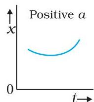
Given that velocity is a vector quantity possessing both magnitude and direction, any alteration in velocity can stem from a modification in either its magnitude, its direction, or a combination of both. Consequently, acceleration can arise from a change in speed (the magnitude of velocity), a change in the direction of motion, or simultaneous changes in both attributes. Analogous to velocity, acceleration can assume positive, negative, or zero values. The corresponding position-time graphs for motion characterized by positive, negative, and zero acceleration are depicted in Figures 2.4 (a), (b), and (c), respectively. It is noteworthy that a graph exhibiting an upward curvature signifies positive acceleration, a downward curvature indicates negative acceleration, and a straight line corresponds to zero acceleration.
While acceleration is generally subject to temporal variation, the scope of our analysis within this chapter will be confined to motion exhibiting constant acceleration. Under this specific condition, the average acceleration over any interval is equivalent to the constant acceleration value throughout that interval. If an object's initial velocity is $v_0$ at time $t = 0$ and its velocity becomes $v$ at a subsequent time $t$, then we can state:
$ \bar {a} = \frac {v - v _ {0}}{t - 0} \text { or } v = v _ {0} + a t \tag {2.4} $
 (a)
(a)
(b)
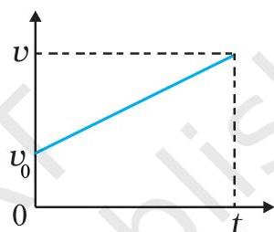
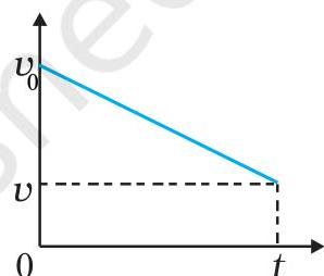
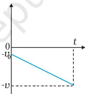
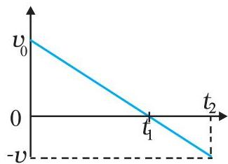
We shall now examine the appearance of velocity-time graphs for several straightforward scenarios. Figure 2.3 illustrates the velocity-time graphs corresponding to motion characterized by constant acceleration under the subsequent conditions:
- (a) An object is moving in a positive direction with a positive acceleration.
- (b) An object is moving in positive direction with a negative acceleration.
- (c) An object is moving in negative direction with a negative acceleration.
- (d) An object is moving in positive direction till time $t_1$, and then turns back with the same negative acceleration.
The area beneath the curve on a velocity-time graph for an object in motion invariably signifies the displacement occurring within a specified time period. While a comprehensive demonstration of this principle necessitates calculus, its validity can be readily observed in the straightforward scenario of an object maintaining a constant velocity $u$. The corresponding velocity-time graph for such movement is depicted in Fig. 2.4.
 (a)
(a)
 (b)
(b)
 (c)
Fig. 2.3 Velocity-time graphs illustrating motion under constant acceleration. (a) Movement in the positive direction with positive acceleration. (b) Movement in the positive direction with negative acceleration. (c) Movement in the negative direction with negative acceleration. (d) Movement of an object experiencing negative acceleration, where its direction reverses at time $t_1$. From time 0 to $t_1$, the object travels in the positive $x$-direction, and from $t_1$ to $t_2$, it proceeds in the opposing direction.
(c)
Fig. 2.3 Velocity-time graphs illustrating motion under constant acceleration. (a) Movement in the positive direction with positive acceleration. (b) Movement in the positive direction with negative acceleration. (c) Movement in the negative direction with negative acceleration. (d) Movement of an object experiencing negative acceleration, where its direction reverses at time $t_1$. From time 0 to $t_1$, the object travels in the positive $x$-direction, and from $t_1$ to $t_2$, it proceeds in the opposing direction.
 (d)
(d)
MOTION IN A STRAIGHT LINE
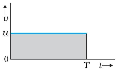 Fig. 2.4 The region beneath the $v - t$ curve corresponds to the object's displacement during a specified time interval.
In the depicted scenario, the $v - t$ curve manifests as a linear segment extending parallel to the temporal axis. The enclosed area beneath this line, bounded by $t = 0$ and $t = T$, constitutes a rectangle with a height of $u$ and a base of $T$. Consequently, the calculation for this area yields $\text{area} = u \times T = uT$, which precisely represents the displacement achieved during this specific time span. It prompts the question: how can a geometric area equate to a physical distance in this context? Consider carefully! By examining the dimensional units of the quantities plotted on both coordinate axes, one can deduce the rationale.
It is important to observe that the position-time ($x - t$), velocity-time ($v - t$), and acceleration-time ($a - t$) graphs presented across various illustrations within this chapter exhibit abrupt changes in slope, or "kinks," at certain junctures. This graphical characteristic signifies that the underlying functions are non-differentiable at these specific points. However, within the context of any actual physical scenario, these functions would consistently be differentiable across all points, resulting in inherently smooth graphical representations.
From a physical perspective, this implies that neither acceleration nor velocity can undergo instantaneous, abrupt alterations in their values. Instead, all such transitions invariably occur in a continuous manner.
2.4 KINEMATIC EQUATIONS FOR UNIFORMLY ACCELERATED MOTION
Under conditions of uniform acceleration, a series of fundamental equations can be formulated to interrelate displacement $(x)$, elapsed time $(t)$, initial velocity $(v_0)$, final velocity $(v)$, and acceleration $(a)$. Equation (2.4), previously established, defines the relationship between the final velocity $v$ and initial velocity $v_0$ for an object undergoing constant acceleration $a$:
$ v = v _ {0} + a t \tag {2.4} $
This relationship is visually depicted in Fig. 2.5. The total area beneath this curve can be determined by summing the area of triangle ABC and the area of rectangle OACD, covering the interval from instant 0 to instant $t$:
$ = \frac {1}{2} (v - v _ {0}) t + v _ {0} t $
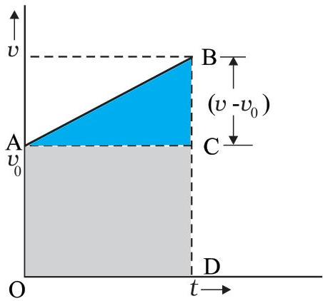 Fig. 2.5 Area under $v - t$ curve for an object with uniform acceleration.
As previously established, the area beneath a velocity-time ($v-t$) graph signifies displacement. Consequently, the displacement $x$ of the object is given by:
$ x = \frac {1}{2} (v - v _ {0}) t + v _ {0} t \tag {2.5} $
Since $v - v_0 = at$, substituting this equivalence into the preceding formula results in $x = \frac{1}{2} a t^2 + v_0 t$, which is conventionally presented as
$x = v_{0}t + \frac{1}{2} at^{2}$ (2.6)
Equation (2.5) may also be expressed in an alternative form:
$ x = \frac {v + v _ {0}}{2} t = \bar {v} t \tag {2.7a} $
where,
$ \bar {v} = \frac {v + v _ {0}}{2} \quad (\text {constant acceleration only}) \tag {2.7b} $
Equations (2.7a) and (2.7b) imply that the object has covered a displacement $x$ with an effective average velocity equivalent to the arithmetic mean of its initial and final velocities.
From Equation (2.4), we can isolate $t$ as $t = (v - v_0) / a$. Substituting this expression for $t$ into Equation (2.7a) leads to:
$ x = \bar {v} t = \left(\frac {v + v _ {0}}{2}\right) \left(\frac {v - v _ {0}}{a}\right) = \frac {v ^ {2} - v _ {0} ^ {2}}{2 a} $
$ v ^ {2} = v _ {0} ^ {2} + 2 a x \tag {2.8} $
This particular equation can also be derived by inserting the value of $t$ from Equation (2.4) into Equation (2.6). Consequently, we have established three pivotal equations:
$ v = v _ {0} + a t $
$ x = v _ {0} t + \frac {1}{2} a t ^ {2} $
$ v ^ {2} = v _ {0} ^ {2} + 2 a x \tag {2.9a} $
These equations establish connections among the five kinematic variables: initial velocity ($v_0$), final velocity ($v$), acceleration ($a$), time ($t$), and displacement ($x$). They constitute the kinematic equations for rectilinear motion under constant acceleration.
The set of equations presented in (2.9a) assumes that the particle's initial position, $x$, is zero at time $t = 0$. A more generalized form can be achieved by considering a non-zero initial position coordinate, denoted as $x_0$, at $t = 0$. In this scenario, Equations (2.9a) are modified by replacing $x$ with $(x - x_0)$ to become:
$ v = v _ {0} + a t $
$ x = x _ {0} + v _ {0} t + \frac {1}{2} a t ^ {2} \tag {2.9b} $
$ v ^ {2} = v _ {0} ^ {2} + 2 a \left(x - x _ {0}\right) \tag {2.9c} $
Example 2.2 Obtain equations of motion for constant acceleration using method of calculus.
Answer By definition, acceleration is the rate of change of velocity:
$ a = \frac {\mathrm {d} v}{\mathrm {d} t} $
Rearranging this, we get:
$ \mathrm {d} v = a \mathrm {d} t $
Integrating both sides of this expression from the initial velocity $v_0$ to final velocity $v$ and from initial time 0 to final time $t$ yields:
$ \int_ {v _ {0}} ^ {v} \mathrm {d} v = \int_ {0} ^ {t} a \mathrm {d} t $
$ = a \int_ {0} ^ {t} \mathrm {d} t \tag {a is} $
constant)
$ v - v _ {0} = a t $
$ v = v _ {0} + a t $
Additionally,
$ v = \frac {\mathrm {d} x}{\mathrm {d} t} $
$ \mathrm {d} x = v \mathrm {d} t $
Upon integrating both expressions,
$ \int_ {x _ {0}} ^ {x} \mathrm {d} x = \int_ {0} ^ {t} v \mathrm {d} t $
$ = \int_ {0} ^ {t} \left(v _ {0} + a t\right) \mathrm {d} t $
$ x - x _ {0} = v _ {0} t + \frac {1}{2} a t ^ {2} $
$ x = x _ {0} + v _ {0} t + \frac {1}{2} a t ^ {2} $
Alternatively, it is possible to express
$ a = \frac {\mathrm {d} v}{\mathrm {d} t} = \frac {\mathrm {d} v}{\mathrm {d} x} \frac {\mathrm {d} x}{\mathrm {d} t} = v \frac {\mathrm {d} v}{\mathrm {d} x} $
$ \text {or,} v \mathrm {d} v = a \mathrm {d} x $
Subsequently, integrating both members yields,
$ \int_ {v _ {0}} ^ {v} v \mathrm {d} v = \int_ {x _ {0}} ^ {x} a \mathrm {d} x $
$ \frac {v ^ {2} - v _ {0} ^ {2}}{2} = a (x - x _ {0}) $
$ v ^ {2} = v _ {0} ^ {2} + 2 a (x - x _ {0}) $
This methodology offers the benefit of applicability even in scenarios involving non-uniform acceleration.
Subsequently, we will apply these derived equations to analyze several significant instances.
Example 2.3 Consider a ball projected vertically upward from the summit of a multi-story structure, possessing an initial velocity of $20\mathrm{ms}^{-1}$. The launch point is situated $25.0\mathrm{m}$ above the ground. (a) Determine the maximum altitude attained by the ball. (b) Calculate the total duration until the ball impacts the ground. Assume the acceleration due to gravity, $\mathrm{g}$, to be $10\mathrm{ms}^{-2}$.
Answer (a) We establish the $y$-axis in the upward vertical orientation, with its origin at ground level, as depicted in Fig. 2.6.
Given values are $v_{0} = +20 , \mathrm{ms}^{-1}$,
$ a = - g = - 1 0 \mathrm {m s} ^ {- 2}, $
$ v = 0 \mathrm {m s} ^ {- 1} $
To ascertain the height $y$ reached by the ball relative to its launch point, we apply the kinematic equation:
$ v ^ {2} = v _ {0} ^ {2} + 2 a (y - y _ {0}) $
This yields:
$ 0 = (2 0) ^ {2} + 2 (- 1 0) (y - y _ {0}) $
Upon resolution, we find $(y - y_0) = 20\mathrm{m}$.
(b) This segment of the problem permits resolution through two distinct approaches. Close attention should be paid to the methodologies employed.
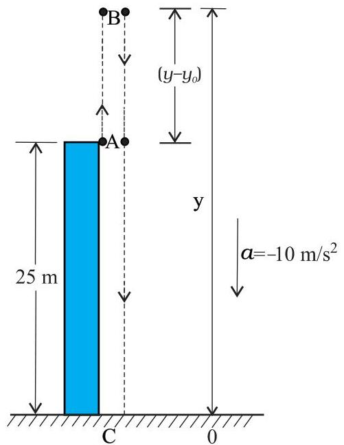 Fig. 2.6
FIRST METHOD: For the initial approach, we segment the trajectory into two distinct phases: the ascent from A to B and the descent from B to C. We then compute the respective durations, $t_1$ and $t_2$. Considering that the velocity at point B is zero, we can state:
$ v = v_0 + a t $
$ 0 = 20 - 10 t_1 $
Or,
$ t_1 = 2 \mathrm{s} $
This value represents the time elapsed during the upward journey from A to B. Subsequent to reaching point B, the apex of its trajectory, the ball undergoes free fall solely influenced by gravitational acceleration. In this phase, the ball's motion is directed along the negative $y$-axis. We utilize the equation:
$ y = y_0 + v_0 t + \frac{1}{2} a t^2 $
Our parameters are $y_0 = 45 \mathrm{m}, y = 0, v_0 = 0, a = -g = -10 \mathrm{m} \mathrm{s}^{-2}$.
$ 0 = 45 + \left(\frac{1}{2}\right) (-10) t_2^2 $
Solving this expression yields $t_2 = 3$ s.
Consequently, the aggregate time until the ball strikes the ground is $t_1 + t_2 = 2\mathrm{s} + 3\mathrm{s} = 5\mathrm{s}$.
ALTERNATIVE APPROACH: The total elapsed time can alternatively be determined by considering the initial and final positional coordinates of the ball relative to a selected origin, in conjunction with the kinematic equation:
$ y = y_0 + v_0 t + \frac{1}{2} a t^2 $
Now $y_0 = 25 \mathrm{m}, y = 0 \mathrm{m}$
$ v_0 = 20 \mathrm{m} \mathrm{s}^{-1}, \quad a = -10 \mathrm{m} \mathrm{s}^{-2}, \quad t = ? $
$ 0 = 25 + 20 t + \left(\frac{1}{2}\right) (-10) t^2 $
Or,
$ 5 t^2 - 20 t - 25 = 0 $
Upon solving this quadratic expression for the variable $t$, the result obtained is:
$ t = 5 \mathrm{s} $
It is worth noting that this alternative method offers an advantage, as it obviates the necessity of analyzing the trajectory of the motion, given that the acceleration remains constant throughout the process.
Example 2.4 Free-fall: Discuss the motion of an object under free fall. Neglect air resistance.
Answer When an object is released in proximity to the Earth's surface, it experiences a downward acceleration resulting from the gravitational force. The symbol $g$ denotes the scalar value of this acceleration due to gravity. The condition where air resistance is disregarded defines what is termed free fall. Provided that the vertical distance covered by the falling object is negligible relative to the Earth's radius, the value of $g$ can be approximated as a constant, specifically $9.8 , \mathrm{m} , \mathrm{s}^{-2}$. Consequently, free fall exemplifies a scenario of motion characterized by uniform acceleration.
For analytical purposes, we posit that the motion occurs along the $y$-axis; more precisely, it proceeds in the negative $y$-direction, as the upward orientation has been designated as positive. Given that gravitational acceleration consistently acts downwards, its vector component aligns with the negative direction, leading to the expression:
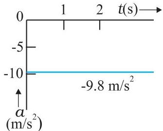
$ a = -g = -9.8 , \mathrm{m} , \mathrm{s}^{-2} $
The object commences its descent from a state of rest at $y = 0$. As a result, the initial velocity $v_0$ is zero, and the governing kinematic equations are transformed into:
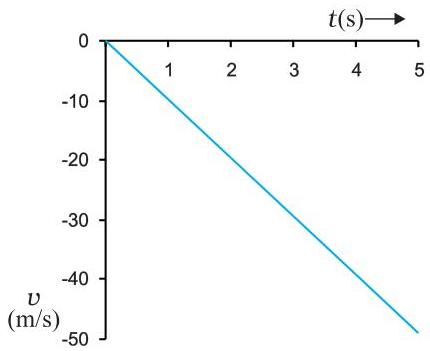
$ v = 0 - g t = -9.8 t , \mathrm{m} , \mathrm{s}^{-1} $
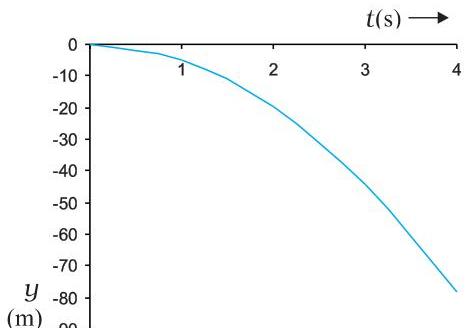
$ y = 0 - \frac{1}{2} g t^2 = -4.9 t^2 , \mathrm{m} $
$ v^2 = 0 - 2 g y = -19.6 y , \mathrm{m}^2 , \mathrm{s}^{-2} $
These formulations yield expressions for both the velocity and the displacement as functions of time, alongside the relationship between velocity and displacement. The temporal dependencies of acceleration, velocity, and displacement are graphically represented in Fig. 2.7(a), (b), and (c), respectively.
 (a)
(a)
(b)
 (c)
Fig. 2.7 Motion of an object under free fall.
(c)
Fig. 2.7 Motion of an object under free fall.
- (a) Variation of acceleration with time.
- (b) Variation of velocity with time.
- (c) Variation of distance with time
Example 2.5 Galileo's law of odd numbers: "The distances traversed, during equal intervals of time, by a body falling from rest, stand to one another in the same ratio as the odd numbers beginning with unity [namely, 1: 3: 5: 7...]." Prove it.
Answer To commence, we partition the total duration of an object's free-fall motion into numerous identical sub-intervals, each of duration $\tau$, for the purpose of determining the respective distances covered.
These are the distances traversed during successive intervals of time. Given an initial velocity of zero, the displacement can be expressed as:
$ y = - \frac {1}{2} g t ^ {2} $
This formula enables the determination of an object's position at various time points, specifically 0, $\tau$, $2\tau$, $3\tau$, and so forth, as detailed in the second column of Table 2.2. If the displacement after the initial time interval $\tau$ is denoted as $y_{it}$, equivalent to $(-1/2)g\tau^2$, then the third column illustrates positions scaled by this $y_{it}$ unit. The fourth column enumerates the distances covered within each sequential interval of $\tau$. Notably, these distances exhibit a straightforward arithmetic progression, specifically a ratio of 1: 3: 5: 7: 9: 11..., as indicated in the final column. This fundamental principle was first articulated by Galileo Galilei (1564-1642), who pioneered the quantitative investigation of objects in free fall.
Example 2.6 Stopping distance of vehicles: The stopping distance refers to the total displacement a moving vehicle undergoes from the moment its brakes are engaged until it comes to a complete halt. This parameter holds significant importance for road safety, being contingent upon the vehicle's initial velocity ($v_{it}$) and the deceleration rate, denoted as $-\alpha$, which is induced by the braking mechanism. Formulate an equation that quantifies the stopping distance of a vehicle as a function of its initial velocity ($v_{it}$) and deceleration ($\alpha$).
Answer Let $d_v$ represent the distance covered by the vehicle prior to cessation. Employing the kinematic equation $v^{2} = v_{0}^{2} + 2ax$ and recognizing that the final velocity $v$ is zero, the stopping distance is ascertained as:
$ d _ {v} = \frac {- v _ {0} ^ {2}}{2 a} $
Consequently, the stopping distance exhibits a direct proportionality to the square of the initial velocity. A twofold increase in the
Table 2.2
| t | y | y in terms of yv [=( - 1/2) g τ2] | Distance traversed in successive intervals | Ratio of distances traversed |
|---|---|---|---|---|
| 0 | 0 | 0 | ||
| τ | -(1/2) g τ2 | yv | yv | 1 |
| 2 τ | -4(1/2) g τ2 | 4 yv | 3 yv | 3 |
| 3 τ | -9(1/2) g τ2 | 9 yv | 5 yv | 5 |
| 4 τ | -16(1/2) g τ2 | 16 yv | 7 yv | 7 |
| 5 τ | -25(1/2) g τ2 | 25 yv | 9 yv | 9 |
| 6 τ | -36(1/2) g τ2 | 36 yv | 11 yv | 11 |
initial velocity results in a quadrupling of the stopping distance, assuming a constant deceleration rate.
Empirical data for a specific vehicle model indicated braking distances of $10\mathrm{m}$, $20\mathrm{m}$, $34\mathrm{m}$, and $50\mathrm{m}$ when initiated from velocities of 11, 15, 20, and $25\mathrm{m/s}$ respectively. These observations demonstrate substantial agreement with the derived formula.
The concept of stopping distance is a critical consideration in the establishment of speed limits, particularly in sensitive areas such as school zones.
Example 2.7 Reaction time: In scenarios necessitating prompt action, a measurable duration elapses prior to an actual response. Reaction time is defined as the interval an individual requires to perceive, process, and initiate an action. For instance, consider a driver encountering an unexpected pedestrian on the road; the time taken from the visual perception of the pedestrian to the initiation of braking constitutes the reaction time. This temporal delay is influenced by both the intricacy of the situation and individual physiological factors.
A straightforward experiment can be conducted to quantify one's reaction time. Have an associate vertically release a ruler such that it falls between your thumb and forefinger (Fig. 2.8). Upon grasping the ruler, measure the distance $d$ it descended. In a specific trial, a value of $21.0 , \text{cm}$ was recorded for $d$. Based on this measurement, calculate the reaction time.
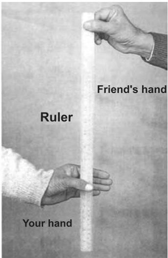 Fig. 2.8 Measuring the reaction time.
Answer In this scenario, the ruler undergoes free fall, implying an initial velocity of $\nu_{a} = 0$ and an acceleration of $a = -g = -9.8 , \mathrm{m} , \mathrm{s}^{-2}$. The relationship between the distance covered, $d$, and the reaction time, $t_{r}$, is established as:
$ d = - \frac {1}{2} g t _ {r} ^ {2} $
Consequently, the reaction time $t_r$ can be expressed as: $t_r = \sqrt{\frac{2d}{g}} , \mathrm{s}$
With a given distance $d = 21.0 , \mathrm{cm}$ and the gravitational acceleration $g = 9.8 , \mathrm{m} , \mathrm{s}^{-2}$, the calculated reaction time is determined to be:
$ t _ {r} = \sqrt {\frac {2 \times 0.21}{9.8}} , \mathrm {s} \cong 0.2 , \mathrm {s}. $
SUMMARY
- Movement is defined by a change in an object's spatial coordinates over time. An object's location is typically defined relative to a selected reference point, or origin. In the context of one-dimensional motion, positions to the right of this origin are conventionally designated as positive, while those to the left are considered negative.
Over a specific time interval, an object's average speed will always be greater than or equal to the absolute value of its average velocity.
- Instantaneous velocity, often referred to simply as velocity, is formally defined as the limiting value of the average velocity as the time increment $\Delta t$ approaches zero:
$ v = \lim _ {\Delta t \rightarrow 0} \bar {v} = \lim _ {\Delta t \rightarrow 0} \frac {\Delta x}{\Delta t} = \frac {\mathrm {d} x}{\mathrm {d} t} $
At any given moment, the velocity corresponds to the gradient of the tangent line on the position-time graph at that precise point.
- The average acceleration represents the ratio of the alteration in velocity to the duration over which this alteration transpires:
$ \overrightarrow {a} = \frac {\Delta v}{\Delta t} $
- Instantaneous acceleration is formally established as the limiting value of the average acceleration as the time interval $\Delta t$ diminishes to zero:
$ a = \lim _ {\Delta t \rightarrow 0} \vec {a} = \lim _ {\Delta t \rightarrow 0} \frac {\Delta v}{\Delta t} = \frac {\mathrm {d} v}{\mathrm {d} t} $
At any specific moment, an object's acceleration is equivalent to the gradient of the velocity-time graph at that precise instant. In the case of uniform motion, acceleration is absent, resulting in an $x - t$ graph that is a straight line angled relative to the time axis, and a $v - t$ graph that appears as a straight line parallel to the time axis. Conversely, for motion characterized by uniform acceleration, the $x - t$ graph takes the form of a parabola, whereas the $v - t$ graph remains a straight line, albeit one that is inclined with respect to the time axis.
- The region encompassed by the velocity-time curve between two specific time points, $t_1$ and $t_2$, quantifies the total displacement experienced by the object throughout that defined temporal span.
- In the context of rectilinear motion with constant acceleration, a fundamental set of relationships, known as the kinematic equations of motion, interlinks five key physical quantities: displacement $x$, elapsed time $t$, initial velocity $v_0$, final velocity $v$, and acceleration $a$:
$ \begin{array}{l} v = v _ {0} + a t \ x = v _ {0} t + \frac {1}{2} a t ^ {2} \ v ^ {2} = v _ {0} ^ {2} + 2 a x \ \end{array} $
These equations are applicable when the object's initial position at $t = 0$ is defined as 0. Should the particle commence its motion from an initial position $x = x_0$, the displacement variable $x$ in the aforementioned equations must be substituted with $(x - x_0)$.
MOTION IN A STRAIGHT LINE
| Physical quantity | Symbol | Dimensions | Unit | Remarks |
|---|---|---|---|---|
| Path length | [L] | m | ||
| Displacement | Δx | [L] | m | $= x_{0} - x_{1}$ In a one-dimensional context, its sign conveys the direction of motion. |
| Velocity | [LT$^{-1}$] | m s$^{-1}$ | ||
| (a) Average | v | $= \frac{\Delta x}{\Delta t}$ | ||
| (b) Instantaneous | v | $= \lim_{\Delta t \to 0} \frac{\Delta x}{\Delta t} = \frac{\mathrm{d}x}{\mathrm{d}t}$ In a one-dimensional context, its sign conveys the direction of |
motion. |
| Speed
(a) Average
(b) Instantaneous | | [LT$^{-1}$] | m s$^{-1}$ | $= \frac{\text{Path length}}{\text{Time interval}}$
$= \frac{\mathrm{d}x}{\mathrm{d}t}$ |
| Acceleration
(a) Average
(b) Instantaneous | $\overline{a}$
$a$ | [LT$^{-2}$] | m s$^{-2}$ | $= \frac{\Delta v}{\Delta t}$
$= \lim_{\Delta t \to 0} \frac{\Delta v}{\Delta t} = \frac{\mathrm{d}v}{\mathrm{d}t}$
In a one-dimensional context, its sign conveys the direction of motion. |
POINTS TO PONDER
- The selection of an axis's origin and its positive orientation is discretionary. This choice must be explicitly established before assigning algebraic signs to physical quantities such as displacement, velocity, and acceleration.
- When a particle's speed increases, its acceleration vector aligns with its velocity vector; conversely, if its speed diminishes, the acceleration vector opposes the velocity vector. This principle remains valid irrespective of the chosen origin or axis orientation.
- The algebraic sign of acceleration does not inherently indicate whether a particle's speed is increasing or decreasing. Rather, the sign of acceleration is determined by the chosen positive direction of the axis. For example, if the upward vertical direction is designated as positive, the acceleration due to gravity is negative. When a particle falls under gravity, this negative acceleration nonetheless causes its speed to increase. Conversely, for a particle projected upwards, the same negative acceleration (from gravity) leads to a decrease in its speed.
- A particle possessing zero velocity at a specific moment does not automatically imply zero acceleration at that same instant. It is possible for a particle to be momentarily stationary while still experiencing non-zero acceleration. An illustrative example is a particle launched vertically upwards, which achieves zero velocity at its peak trajectory, yet its acceleration at that precise moment remains equivalent to the acceleration due to gravity.
- Within the kinematic equations of motion [Eq. (2.9)], the involved quantities are algebraic in nature, meaning they can assume either positive or negative values. These equations are universally valid for one-dimensional motion under constant acceleration, contingent upon the substitution of all quantity values with their appropriate algebraic signs.
- The conceptual definitions of instantaneous velocity and acceleration (Eqs. (2.1) and (2.3)) are fundamentally precise and universally applicable. In contrast, the kinematic equations (Eq. (2.9)) hold true exclusively for motion where both the magnitude and the directional vector of acceleration remain invariant throughout the duration of the motion.
EXERCISES
2.1 For which of the subsequent scenarios of movement
can the object be approximately modeled as a point mass:
- (a) a train car traversing smoothly between two terminals.
- (b) an ape perched on a person pedaling uniformly along a circular path.
- (c) a rotating cricket sphere that deviates abruptly upon impact with the surface.
- (d) an overturning laboratory vessel that has fallen from the perimeter of a desk.
2.2 Figure 2.9 illustrates the position-time $(x - t)$ diagrams for two individuals, A and B, as they journey back from their educational institution O to their respective residences P and Q. Select the appropriate options within the parentheses provided;
- (a) (A/B) resides nearer to the school than (B/A)
- (b) (A/B) commences their departure from school sooner than (B/A)
- (c) (A/B) proceeds on foot at a greater speed than (B/A)
- (d) A and B arrive at their dwelling at the (identical/distinct) time
- (e) (A/B) surpasses (B/A) during their commute (a single instance/two instances).
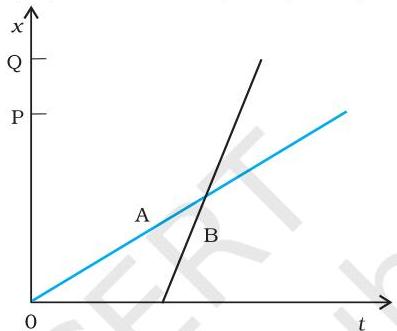 Fig. 2.9
2.3 A female individual departs from her residence at 9:00 AM, traversing on foot at a speed of $5\mathrm{km}\mathrm{h}^{-1}$ along a linear route to her workplace, located $2.5\mathrm{km}$ away. She remains at the office until 5:00 PM, then returns home by an auto-rickshaw at a speed of $25\mathrm{km}\mathrm{h}^{-1}$. Select appropriate scales and delineate the $x - t$ graph of her journey. 2.4 An inebriated individual traversing a constricted pathway progresses 5 strides forward and 3 strides backward, with this pattern subsequently recurring. Each stride measures $1\mathrm{m}$ in length and consumes $1\mathrm{s}$. Illustrate the $x - t$ graph depicting his movement. Ascertain, both by graphical analysis and analytical computation, the time required for the individual to fall into a pit located $13\mathrm{m}$ from his initial position. 2.5 An automobile traveling on a linear thoroughfare at a speed of $126\mathrm{km}\mathrm{h}^{-1}$ is decelerated to a halt within a span of $200\mathrm{m}$. What is the vehicle's deceleration (presumed constant), and what is the duration required for the vehicle to cease motion? 2.6 An athlete propels a sphere vertically upward with an initial velocity magnitude of $29.4 , \text{m} , \text{s}^{-1}$.
- (a) In which orientation does the acceleration act during the projectile's ascent?
- (b) Determine the velocity and acceleration of the sphere at the apex of its trajectory.
- (c) Designate $x = 0 , \text{m}$ and $t = 0 , \text{s}$ as the spatial and temporal coordinates of the sphere at its maximum elevation, with the vertically downward orientation defined as the positive direction for the $x$-axis. Subsequently, specify the algebraic signs of the sphere's position, velocity, and acceleration during its upward and downward phases of movement.
- (d) What is the maximum altitude attained by the sphere, and after what elapsed time does it return to the thrower's grasp? (Assume $g = 9.8 , \text{m} , \text{s}^{-2}$ and disregard atmospheric drag).
2.7 Scrutinize each assertion presented below and indicate, providing justifications and illustrations, whether it holds true or false;
A particle in one-dimensional motion
- (a) possessing zero instantaneous speed may concurrently exhibit non-zero acceleration at that precise moment.
- (b) having no speed may nonetheless possess a non-zero velocity,
- (c) maintaining a constant speed is necessarily indicative of zero acceleration,
- (d) exhibiting a positive acceleration value invariably implies an increase in speed.
MOTION IN A STRAIGHT LINE
2.8 A sphere is released from a vertical elevation of $90,\mathrm{m}$ above a horizontal surface. Upon each impact with the surface, the object's speed diminishes by one-tenth of its current value. Construct a speed-time graph illustrating its trajectory within the time interval from $t = 0$ to $12,\mathrm{s}$.
2.9 Provide a lucid explanation, supported by illustrative instances, differentiating between:
- (a) the absolute value of displacement (occasionally referred to as distance) spanning a given temporal duration, and the aggregate linear extent of the trajectory traversed by a point mass within that identical duration;
- (b) the absolute value of the mean velocity across a specified time interval, and the mean speed over the identical interval. [The mean speed of a point mass over a time interval is formally defined as the cumulative path length divided by the duration of that interval]. For both (a) and (b), demonstrate that the latter quantity is invariably either numerically superior to or equivalent to the former. Under what specific conditions does this equality hold? [To maintain simplicity, confine your analysis to unidirectional motion].
2.10 A pedestrian traverses a linear path from his residence to a marketplace situated $2.5,\mathrm{km}$ distant, proceeding at a constant rate of $5,\mathrm{km},\mathrm{h}^{-1}$. Upon discovering the establishment to be non-operational, he immediately reverses direction and returns to his residence, maintaining a rate of $7.5,\mathrm{km},\mathrm{h}^{-1}$. Determine the following:
- (a) the absolute value of the mean velocity, and
- (b) the mean speed of the individual across the following time intervals: (i) 0 to $30,\mathrm{min}$, (ii) 0 to $50,\mathrm{min}$, (iii) 0 to $40,\mathrm{min}$? [Observe from this problem's analysis why it is more appropriate to conceptualize mean speed as the cumulative path length divided by the elapsed time, rather than as the absolute value of the mean velocity. One would scarcely wish to inform the fatigued individual upon his arrival back home that his mean speed was null!]
2.11 In the preceding Problems 2.9 and 2.10, a meticulous differentiation was established between mean speed and the absolute value of mean velocity. However, such a distinction becomes superfluous when examining instantaneous speed and the absolute value of instantaneous velocity. The instantaneous speed invariably corresponds precisely to the absolute value of the instantaneous velocity. Elucidate the rationale for this phenomenon.
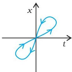
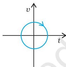
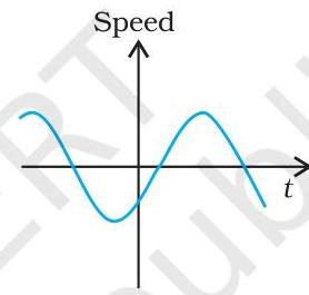
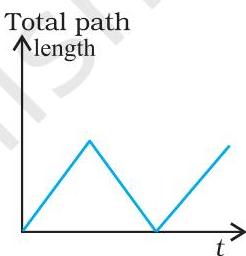
2.12 Scrutinize the provided graphs from (a) to (d) (Fig. 2.10) attentively and articulate, furnishing justifications, which among them are fundamentally incapable of depicting the one-dimensional motion of a particle.
2.13 Figure 2.11 illustrates the $x - t$ representation of a particle's one-dimensional motion. Is it accurate to infer from this graphical representation that the particle executes linear motion for $t < 0$ and follows a parabolic trajectory for $t > 0$? Should this inference be incorrect, propose an appropriate physical scenario that this graph could represent.
2.14 A law enforcement vehicle traversing a thoroughfare at a velocity of $30,\mathrm{km},\mathrm{h}^{-1}$ discharges a projectile towards a getaway vehicle, operated by a suspect, which is accelerating in the identical direction at $192,\mathrm{km},\mathrm{h}^{-1}$. Given that the projectile's muzzle velocity is $150,\mathrm{m},\mathrm{s}^{-1}$, what is the impact speed of the projectile as it strikes the suspect's vehicle? (Note: Calculate the speed that is pertinent to inflicting damage upon the suspect's vehicle).
 (a)
(a)
 (b)
(b)
 (c)
(c)
 (d)
(d)
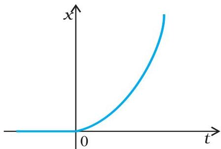 Fig. 2.10
PHYSICS
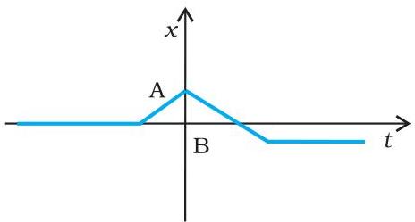
2.15 For each graph presented below (refer to Fig 2.12), describe a corresponding appropriate physical scenario:
 (a)
(a)
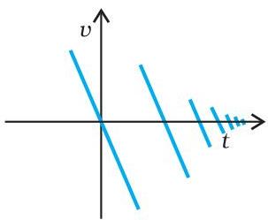 (b)
(b)
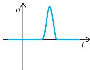 (c)
(c)
2.16 The $x-t$ plot shown in Figure 2.13 illustrates the motion of a particle undergoing one-dimensional simple harmonic oscillation. (Further details regarding this motion will be covered in Chapter 13). Determine the signs of the position, velocity, and acceleration variables for the particle at the time instants $t = 0.3$ s, $1.2$ s, and $-1.2$ s.
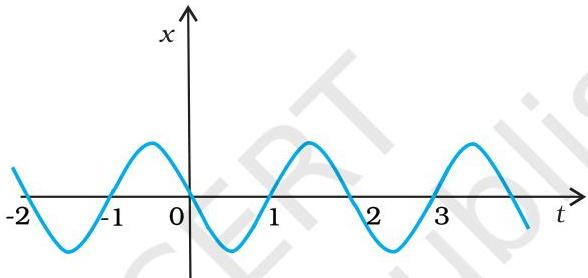 Fig. 2.12
2.17 The $x-t$ graph in Figure 2.14 depicts the one-dimensional motion of a particle. It displays three distinct time intervals of equal duration. Identify the interval where the average speed is maximal and the interval where it is minimal. State the sign of the average velocity for each of these intervals.
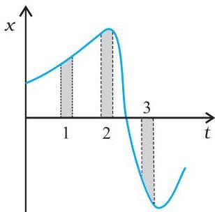 Fig. 2.13
2.18 Figure 2.15 presents a speed-time graph illustrating the movement of a particle along a consistent direction. Three time intervals of identical length are indicated. Which interval exhibits the largest magnitude for average acceleration? Which interval corresponds to the highest average speed? Assuming the constant direction of motion is positive, specify the signs of velocity ($v$) and acceleration ($a$) within each of the three intervals. Determine the acceleration values at points A, B, C, and D.
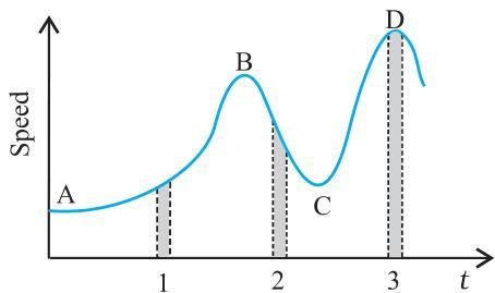 Fig. 2.14
Fig. 2.15
Fig. 2.14
Fig. 2.15