CHAPTER THREE
MOTION IN A PLANE
3.1 Introduction
3.2 Scalars and vectors
3.3 Multiplication of vectors by real numbers
3.4 Addition and subtraction of vectors — graphical method
3.5 Resolution of vectors
3.6 Vector addition — analytical method
3.7 Motion in a plane
3.8 Motion in a plane with constant acceleration
3.9 Projectile motion
3.10 Uniform circular motion
Summary
Points to ponder
Exercises
3.1 INTRODUCTION
The preceding chapter introduced the foundational concepts of position, displacement, velocity, and acceleration, which are essential for characterizing an object's linear motion. It was established that in one-dimensional scenarios, the directional attribute of these quantities could be adequately represented using positive and negative signs, given the limited possibility of only two opposing directions. However, to accurately depict the motion of an object in a two-dimensional plane or three-dimensional space, the application of vectors becomes indispensable for defining these physical magnitudes. Consequently, a preliminary understanding of vector algebra is imperative. This includes addressing fundamental questions such as the definition of a vector, the methodologies for vector addition, subtraction, and multiplication, and the implications of scaling a vector by a real number. Acquiring this knowledge will equip us to effectively employ vectors in the formulation of velocity and acceleration within a planar context. Subsequently, the dynamics of an object moving within a plane will be examined. As a specific instance of planar motion, uniform acceleration will be analyzed, with a comprehensive treatment of projectile motion. Furthermore, circular motion, a ubiquitous phenomenon with considerable practical relevance, will be explored, focusing particularly on uniform circular motion.
The mathematical formulations derived within this chapter concerning motion in a plane are readily extensible to encompass three-dimensional scenarios.
3.2 SCALARS AND VECTORS
In the realm of physics, quantities are categorized into two fundamental types: scalars and vectors. The primary distinction lies in the fact that a vector possesses an associated direction, whereas a scalar does not. A scalar quantity is characterized solely by its magnitude. Its complete specification requires only a numerical value, accompanied by the appropriate unit. Illustrative examples include: the spatial separation between two points, an object's mass, the thermal state of a body (temperature), and the temporal point at which a specific event occurs. The operational rules for combining scalar quantities align with those of conventional algebra. Scalars are amenable to addition, subtraction, multiplication, and division, mirroring the arithmetic operations applied to
ordinary numbers. For instance, consider a rectangle with a length of 1.0 m and a breadth of 0.5 m. Its perimeter is determined by summing the lengths of its four sides: 1.0 m + 0.5 m + 1.0 m + 0.5 m = 3.0 m. Here, the length of each side is a scalar, and the resulting perimeter is also a scalar. To offer another illustration, if the highest and lowest temperatures recorded on a particular day are 35.6 °C and 24.2 °C, respectively, then their difference is 11.4 °C. Similarly, if a uniform solid aluminum cube with a side length of 10 cm has a mass of 2.7 kg, its volume is 10⁻³ m³ (a scalar), and its density is 2.7×10³ kg m⁻³ (also a scalar).
A vector quantity is defined as a quantity possessing both a magnitude and a direction, and which adheres to the triangle law of addition, or equivalently, the parallelogram law of addition. Consequently, a vector is fully characterized by providing its numerical magnitude and its specified direction. Examples of physical quantities represented by vectors include displacement, velocity, acceleration, and force.
Within the context of this text, vectors are denoted using boldface type. Thus, a velocity vector might be represented by the symbol v. Given the practical difficulty of rendering boldface in handwritten contexts, a vector is frequently indicated by placing an arrow above a letter, for instance, $\vec{v}$. Therefore, both v and $\vec{v}$ serve to represent the velocity vector. The magnitude of a vector is commonly referred to as its absolute value, symbolized as |v| = v. Hence, a vector is typically presented in boldface, such as A, a, p, q, r, ... x, y, with their corresponding magnitudes indicated by lightface characters: A, a, p, q, r, ... x, y.
3.2.1 Position and Displacement Vectors
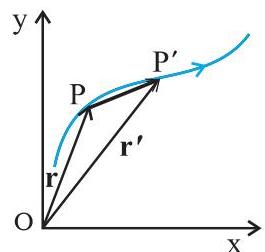
To define the spatial location of an object traversing a plane, one must first select a convenient reference point, typically denoted as the origin O. Let the object's positions at times t and t' be P and P', respectively, as illustrated in [Fig. 3.1(a)]. The straight line segment drawn from O to P constitutes the position vector of the object at time t. This vector is visually indicated by an arrow at its terminus and is represented by the symbol r, such that OP = r. Correspondingly, P' is represented by a different position vector, OP', symbolized as r'. The length of the vector r signifies its magnitude, and its orientation specifies the direction of P when viewed from O. Should the object transition from point P to P', the vector PP'—originating at P and terminating at P'—is termed the displacement vector. This vector describes the change in position from point P (at time t) to P' (at time t').
 (a)
(a)
 (b)
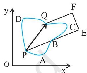
Fig. 3.1 (a) Position and displacement vectors. (b) Displacement vector PQ and different courses of motion.
(b)
Fig. 3.1 (a) Position and displacement vectors. (b) Displacement vector PQ and different courses of motion.
It is crucial to recognize that the displacement vector is solely defined by the direct line segment connecting the initial and final points, and it remains unaffected by the specific trajectory or path followed by the object between these two positions. For instance, as shown in Fig. 3.1(b), if P and Q represent the initial and final positions, the displacement vector PQ remains identical regardless of the actual paths taken, such as PABCQ, PDQ, or PBEFQ. Consequently, the magnitude of the displacement is always less than or, in the case of a straight-line path without reversal, equal to the total path length covered by the object between the two points. This principle was also highlighted in the preceding chapter during the discussion of one-dimensional motion.
3.2.2 Equality of Vectors
Two vectors, A and B, are defined as equal if, and only if, they possess identical magnitudes and precisely the same direction.
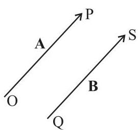
Figure 3.2(a) illustrates two equal vectors, A and B. Their equivalence can be verified through a simple geometric operation. By translating vector B without altering its orientation, such that its initial point (Q) aligns with the initial point (O) of vector A, if their terminal points (S and P) also coincide, then the two vectors are confirmed as equal. This equivalence is conventionally represented as $\mathbf{A} = \mathbf{B}$.
 (a)
(a)
 (b)
Fig. 3.2 (a) Two equal vectors $\mathbf{A}$ and $\mathbf{B}$. (b) Two vectors $\mathbf{A}'$ and $\mathbf{B}'$ are unequal though they are of the same length.
(b)
Fig. 3.2 (a) Two equal vectors $\mathbf{A}$ and $\mathbf{B}$. (b) Two vectors $\mathbf{A}'$ and $\mathbf{B}'$ are unequal though they are of the same length.
Conversely, as illustrated in Figure 3.2(b), vectors $\mathbf{A}'$ and $\mathbf{B}'$, despite possessing identical magnitudes, are not considered equal due to their divergent directions. Should $\mathbf{B}'$ be translated parallel to its initial orientation such that its origin, $Q'$, aligns with the origin, $O'$, of $\mathbf{A}'$, their respective terminal points, $S'$ and $P'$, would fail to coincide.
3.3 MULTIPLICATION OF VECTORS BY REAL NUMBERS
When a vector $\mathbf{A}$ is scaled by a positive real number $\lambda$, the resulting vector's magnitude is altered by a factor of $\lambda$, while its orientation remains identical to that of $\mathbf{A}$:
$ \left| \lambda \mathbf {A} \right| = \lambda \left| \mathbf {A} \right| \text {i f} \lambda > 0. $
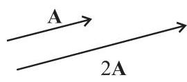
For instance, if vector $\mathbf{A}$ undergoes multiplication by 2, the resultant vector, denoted as $2\mathbf{A}$, maintains the same direction as $\mathbf{A}$ but possesses a magnitude that is twice the magnitude of $|\mathbf{A}|$, as illustrated in Fig. 3.3(a).
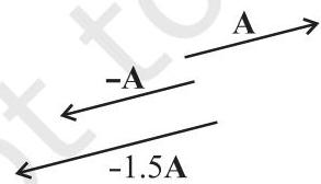
Conversely, multiplying a vector $\mathbf{A}$ by a negative real number, such as $-\lambda$, yields a new vector whose direction is precisely opposite to that of $\mathbf{A}$, and whose magnitude is $\lambda$ times the magnitude of $|\mathbf{A}|$.
Vectors obtained by multiplying a given vector $\mathbf{A}$ by negative numerical values, for example -1 and -1.5, are depicted in Fig 3.3(b).
 (a)
(a)
 (b)
(b)
The scalar factor $\lambda$ used to multiply vector $\mathbf{A}$ may possess its own distinct physical dimension. In such instances, the dimension of the product $\lambda \mathbf{A}$ is derived from the product of the dimensions of $\lambda$ and $\mathbf{A}$. For example, the product of a constant velocity vector and a duration (representing time) results in a displacement vector.
3.4 ADDITION AND SUBTRACTION OF VECTORS — GRAPHICAL METHOD
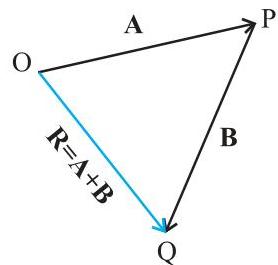
As established in section 4.2, vectors inherently conform to the triangle law of addition, which is synonymous with the parallelogram law. The graphical approach to elucidating this principle of vector summation will now be presented. Imagine two vectors, $\mathbf{A}$ and $\mathbf{B}$, situated within a common plane, as depicted in Fig. 3.4(a). The dimensions of the linear segments symbolizing these vectors maintain a direct proportionality to their respective magnitudes. To determine the resultant $\mathbf{A} + \mathbf{B}$, one positions vector $\mathbf{B}$ such that its origin coincides with the terminus of vector $\mathbf{A}$, as illustrated in Fig. 3.4(b). Subsequently, a line is drawn connecting the origin of $\mathbf{A}$ to the terminus of $\mathbf{B}$. This segment, denoted OQ, constitutes the vector $\mathbf{R}$, which signifies the aggregate of vectors $\mathbf{A}$ and $\mathbf{B}$. Given that, within this methodology for combining vectors, the vectors are
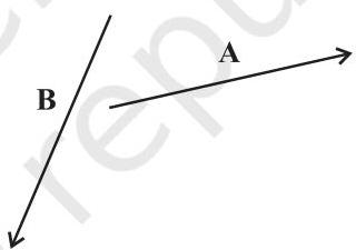 Fig. 3.3 (a) Vector $\mathbf{A}$ and the resultant vector after multiplying $\mathbf{A}$ by a positive number 2. (b) Vector $\mathbf{A}$ and resultant vectors after multiplying it by a negative number -1 and -1.5.
(a)
Fig. 3.3 (a) Vector $\mathbf{A}$ and the resultant vector after multiplying $\mathbf{A}$ by a positive number 2. (b) Vector $\mathbf{A}$ and resultant vectors after multiplying it by a negative number -1 and -1.5.
(a)
 (b)
(b)
 (c)
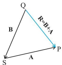
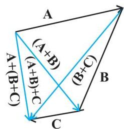
Fig. 3.4 (a) Vectors $\mathbf{A}$ and $\mathbf{B}$ . (b) Vectors $\mathbf{A}$ and $\mathbf{B}$ added graphically. (c) Vectors $\mathbf{B}$ and $\mathbf{A}$ added graphically. (d) Illustrating the associative law of vector addition.
(c)
Fig. 3.4 (a) Vectors $\mathbf{A}$ and $\mathbf{B}$ . (b) Vectors $\mathbf{A}$ and $\mathbf{B}$ added graphically. (c) Vectors $\mathbf{B}$ and $\mathbf{A}$ added graphically. (d) Illustrating the associative law of vector addition.
 (d)
(d)
aligned in a head-to-tail fashion, this visual technique is consequently termed the head-to-tail method. Given that the initial two vectors and their combined outcome delineate the three sides of a triangle, this approach is alternatively referred to as the triangle method for vector combination. Should one determine the resultant of $\mathbf{B} + \mathbf{A}$, as demonstrated in Fig. 3.4(c), the identical vector $\mathbf{R}$ will manifest. This observation establishes the commutative property of vector addition:
$ \mathbf {A} + \mathbf {B} = \mathbf {B} + \mathbf {A} \tag {3.1} $
Furthermore, the summation of vectors adheres to the associative law, as depicted in Fig. 3.4(d). The aggregate achieved by first combining vectors $\mathbf{A}$ and $\mathbf{B}$ and subsequently incorporating vector $\mathbf{C}$ is equivalent to the aggregate derived from initially combining vectors $\mathbf{B}$ and $\mathbf{C}$ and then incorporating vector $\mathbf{A}$:
$ (\mathbf {A} + \mathbf {B}) + \mathbf {C} = \mathbf {A} + (\mathbf {B} + \mathbf {C}) \tag {3.2} $
What outcome arises from the summation of two vectors that are equal in magnitude but opposite in direction? Examine the pair of vectors, $\mathbf{A}$ and $-\mathbf{A}$, presented in Fig. 3.3(b). Their collective sum is expressed as $\mathbf{A} + (-\mathbf{A})$. Because these two vectors possess identical magnitudes but divergent directions, their resultant vector exhibits a magnitude of zero and is symbolized by $\mathbf{0}$, known as a null vector or a zero vector:
$ \mathbf {A} - \mathbf {A} = \mathbf {0} \quad | \mathbf {0} | = 0 \tag {3.3} $
Given that a null vector possesses a magnitude of zero, its directional orientation remains undefined. Furthermore, a null vector is generated when any vector $\mathbf{A}$ is scaled by the scalar quantity zero. The primary characteristics of $\mathbf{0}$ include:
$ \mathbf {A} + \mathbf {0} = \mathbf {A} $
$ \lambda \mathbf {0} = \mathbf {0} $
$ 0 \mathbf {A} = \mathbf {0} \tag {3.4} $
 (a)
(a)
To elucidate the physical significance of a zero vector, let us examine position and displacement vectors within a planar context, as depicted in Fig. 3.1(a). Imagine an object initially located at point $\mathbf{P}$ at time $t$. If this object subsequently translates to point $\mathbf{P}'$ and then returns precisely to its original position $\mathbf{P}$, its net displacement is then considered. Given the congruence of the initial and final spatial coordinates, the resultant displacement is identified as a "null vector."
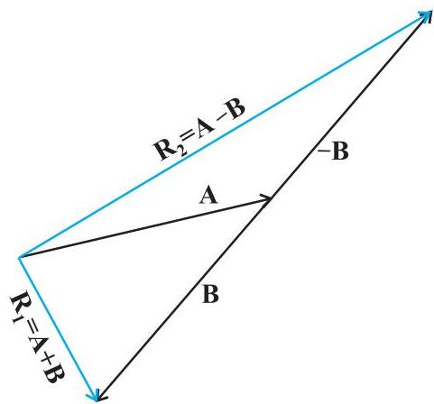
The operation of vector subtraction can be conceptualized as an extension of vector addition. Specifically, the difference between two vectors, $\mathbf{A}$ and $\mathbf{B}$, is formally defined as the sum of vector $\mathbf{A}$ and the negative of vector $\mathbf{B}$:
$ \mathbf {A} - \mathbf {B} = \mathbf {A} + (- \mathbf {B}) \tag {3.5} $
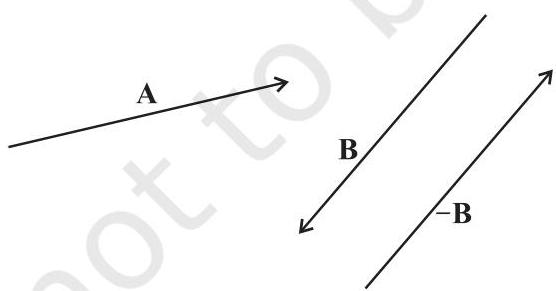
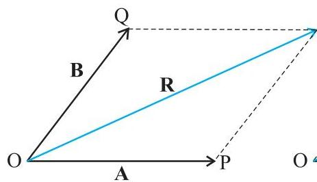
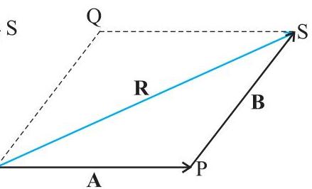
This concept is visually represented in Fig 3.5. Here, vector $-\mathbf{B}$ is graphically combined with vector $\mathbf{A}$ to yield the resultant $\mathbf{R}_2 = (\mathbf{A} - \mathbf{B})$. For comparative purposes, the sum of vectors $\mathbf{A}$ and $\mathbf{B}$, denoted as $\mathbf{R}_1 = \mathbf{A} + \mathbf{B}$, is also illustrated within the same diagram. An alternative approach for determining the sum of two vectors involves the parallelogram method. Consider two arbitrary vectors, $\mathbf{A}$ and $\mathbf{B}$. To perform their addition, their initial points (tails) are aligned at a shared origin, designated $\mathbf{O}$, as depicted in Fig. 3.6(a). Subsequently, a line segment is extended from the terminus (head) of $\mathbf{A}$, drawn parallel to $\mathbf{B}$, and similarly, another line segment is extended from the terminus of $\mathbf{B}$, drawn parallel to $\mathbf{A}$. These parallel lines form a parallelogram, typically labeled OQSP. The resultant vector $\mathbf{R}$ is then established by connecting the common origin $\mathbf{O}$ to the intersection point of these two parallel lines, thereby forming the diagonal (OS) of the parallelogram, as shown in [Fig. 3.6(b)]. Furthermore, Fig. 3.6(c) demonstrates the application of the triangle law for vector addition to obtain the resultant of $\mathbf{A}$ and $\mathbf{B}$, confirming that both methodologies produce an identical outcome. Consequently, these two methods are demonstrably equivalent.
 (b)
Fig. 3.5 (a) Two vectors $\mathbf{A}$ and $\mathbf{B}$, $-\mathbf{B}$ is also shown. (b) Subtracting vector $\mathbf{B}$ from vector $\mathbf{A}$ – the result is $\mathbf{R}_2$. For comparison, addition of vectors $\mathbf{A}$ and $\mathbf{B}$, i.e. $\mathbf{R}_1$ is also shown.
(b)
Fig. 3.5 (a) Two vectors $\mathbf{A}$ and $\mathbf{B}$, $-\mathbf{B}$ is also shown. (b) Subtracting vector $\mathbf{B}$ from vector $\mathbf{A}$ – the result is $\mathbf{R}_2$. For comparison, addition of vectors $\mathbf{A}$ and $\mathbf{B}$, i.e. $\mathbf{R}_1$ is also shown.
 (a)
(a)
 (b)
(b)
 (c)
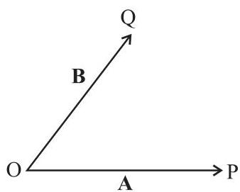
Fig. 3.6 (a) Two vectors $\mathbf{A}$ and $\mathbf{B}$ with their tails brought to a common origin. (b) The sum $\mathbf{A} + \mathbf{B}$ obtained using the parallelogram method. (c) The parallelogram method of vector addition is equivalent to the triangle method.
(c)
Fig. 3.6 (a) Two vectors $\mathbf{A}$ and $\mathbf{B}$ with their tails brought to a common origin. (b) The sum $\mathbf{A} + \mathbf{B}$ obtained using the parallelogram method. (c) The parallelogram method of vector addition is equivalent to the triangle method.
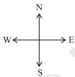
Example 3.1 Rain is falling vertically with a speed of $35\mathrm{ms}^{-1}$. Wind starts blowing after sometime with a speed of $12\mathrm{ms}^{-1}$ in east to west direction. In which direction should a boy waiting at a bus stop hold his umbrella?
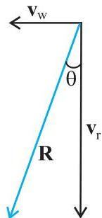 Fig. 3.7
Answer As illustrated in Fig. 3.7, the velocities of the rain and the wind are denoted by the vectors $\mathbf{v}{\mathrm{r}}$ and $\mathbf{v}{\mathrm{w}}$, respectively, corresponding to the directions specified in the problem statement. By applying the principles of vector addition, the resultant vector of $\mathbf{v}{\mathrm{r}}$ and $\mathbf{v}{\mathrm{w}}$ is determined to be $\mathbf{R}$, as depicted in the figure. The magnitude of this resultant, $\mathbf{R}$, is calculated as follows:
$ R = \sqrt {v _ {r} ^ {2} + v _ {w} ^ {2}} = \sqrt {3 5 ^ {2} + 1 2 ^ {2}} \mathrm {m s} ^ {- 1} = 3 7 \mathrm {m s} ^ {- 1} $
The angular orientation $\theta$ of $\mathbf{R}$ with respect to the vertical axis is given by:
$ \tan \theta = \frac {v _ {w}}{v _ {r}} = \frac {1 2}{3 5} = 0. 3 4 3 $
Or, $\theta = \tan^{-1}(0.343) = 19^{\circ}$
Consequently, the boy should position his umbrella within the vertical plane at an approximate angle of $19^{\circ}$ relative to the vertical, oriented towards the east.
3.5 RESOLUTION OF VECTORS
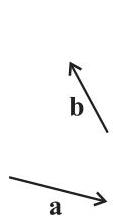
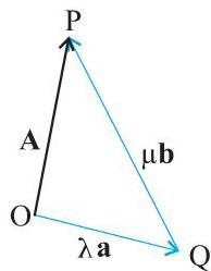
Consider two non-zero vectors, $\mathbf{a}$ and $\mathbf{b}$, situated within a given plane, possessing distinct orientations. Let $\mathbf{A}$ represent an additional vector residing in this identical plane (refer to Fig. 3.8). It is possible to articulate $\mathbf{A}$ as the composite sum of two constituent vectors: one derived from scaling $\mathbf{a}$ by a real scalar, and the other from scaling $\mathbf{b}$ by a distinct real scalar. To illustrate this principle, designate $\mathrm{O}$ as the initial point and $\mathrm{P}$ as the terminal point of vector $\mathbf{A}$. Subsequently, construct a line originating from $\mathrm{O}$ that runs parallel to $\mathbf{a}$, and another line originating from $\mathrm{P}$ that runs parallel to $\mathbf{b}$. Let the intersection of these two lines be denoted by $\mathrm{Q}$. Consequently, we establish the relation:
$ \mathbf {A} = \mathbf {O P} = \mathbf {O Q} + \mathbf {Q P} \tag {3.6} $
Given that $\mathbf{OQ}$ aligns parallel to $\mathbf{a}$, and $\mathbf{QP}$ aligns parallel to $\mathbf{b}$, it follows that we can express these relationships as:
$ \mathbf {O Q} = \lambda \mathbf {a}, \text {and} \mathbf {Q P} = \mu \mathbf {b} \tag {3.7} $
where $\lambda$ and $\mu$ are real numbers.
Therefore, $\mathbf{A} = \lambda \mathbf{a} + \mu \mathbf{b}$ (3.8)
 (a)
(a)
 (b)
Fig. 3.8 (a) Two non-colinear vectors $\mathbf{a}$ and $\mathbf{b}$ . (b) Resolving a vector $\mathbf{A}$ in terms of vectors $\mathbf{a}$ and $\mathbf{b}$ .
(b)
Fig. 3.8 (a) Two non-colinear vectors $\mathbf{a}$ and $\mathbf{b}$ . (b) Resolving a vector $\mathbf{A}$ in terms of vectors $\mathbf{a}$ and $\mathbf{b}$ .
The vector $\mathbf{A}$ is thus characterized as having been decomposed into two constituent vectors, specifically $\lambda \mathbf{a}$ and $\mu \mathbf{b}$, aligned with the directions of $\mathbf{a}$ and $\mathbf{b}$ respectively. This methodology permits the decomposition of any arbitrary vector into a pair of component vectors, provided all three
vectors reside within the same plane. For practical applications, it is often more advantageous to decompose a general vector along the orthogonal axes of a Cartesian coordinate system, employing vectors possessing a magnitude of one. These specialized vectors are termed unit vectors, a concept we will now elaborate upon. A unit vector is fundamentally defined as a vector with a magnitude of one, serving solely to indicate a specific direction. It inherently lacks any physical dimension or associated unit. Its sole purpose is directional specification. Within a rectangular coordinate system, the unit vectors corresponding to the $x$-, $y$-, and $z$-axes are conventionally represented by $\hat{\mathbf{i}}$, $\hat{\mathbf{j}}$, and $\hat{\mathbf{k}}$, respectively, as depicted in Fig. 3.9(a).
Since these are unit vectors, we have
$ \left| \hat {\mathbf {i}} \right| = \left| \hat {\mathbf {j}} \right| = \left| \hat {\mathbf {k}} \right| = 1 \tag {3.9} $
These unit vectors exhibit mutual orthogonality. Within the scope of this document, they are rendered in boldface typography, surmounted by a circumflex accent (^) to differentiate them from other vector quantities. Given that the current chapter focuses on kinematics in two dimensions, our analysis will necessitate the employment of only two such unit vectors. When a unit vector, for instance $\hat{\mathbf{n}}$, undergoes multiplication by a scalar quantity, the outcome is a resultant vector
$\hat{\lambda} = \lambda \hat{\mathbf{n}}$ In general, a vector $\mathbf{A}$ can be written as
$ \mathbf {A} = | \mathbf {A} | \hat {\mathbf {n}} \tag {3.10} $
where $\hat{\mathbf{n}}$ is a unit vector along $\mathbf{A}$.
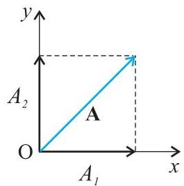
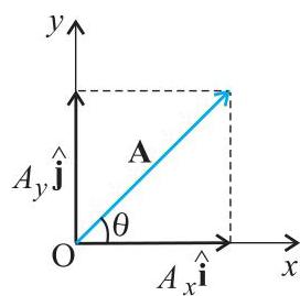
The decomposition of a vector $\mathbf{A}$ into component vectors aligned with the unit vectors $\hat{\mathbf{i}}$ and $\hat{\mathbf{j}}$ can now be performed. Consider a vector $\mathbf{A}$ situated within the $x-y$ plane, as depicted in Fig. 3.9(b). By projecting lines perpendicularly from the terminus of $\mathbf{A}$ onto the coordinate axes, as illustrated in Fig. 3.9(b), we derive vectors $\mathbf{A}_1$ and $\mathbf{A}_2$ such that their vector sum equals $\mathbf{A}$ ($\mathbf{A}_1 + \mathbf{A}_2 = \mathbf{A}$). Given that $\mathbf{A}_1$ is collinear with $\hat{\mathbf{i}}$ and $\mathbf{A}_2$ is collinear with $\hat{\mathbf{j}}$, the following relationships hold:
$ \mathbf {A} _ {1} = A _ {x} \hat {\mathbf {i}}, \quad \mathbf {A} _ {2} = A _ {y} \hat {\mathbf {j}} \tag {3.11} $
where $A_{x}$ and $A_{y}$ denote scalar real numbers.
Consequently, $\mathbf{A} = A_{x}\hat{\mathbf{i}} +A_{y}\hat{\mathbf{j}}$ (3.12). This formulation is visually presented in Fig. 3.9(c). The scalar quantities $A_{x}$ and $A_{y}$ are designated as the $x$-component and $y$-component of vector $\mathbf{A}$, respectively. It is crucial to distinguish that $A_{x}$ itself is a scalar, whereas $A_{x}\hat{\mathbf{i}}$ constitutes a vector, as does $A_{y}\hat{\mathbf{j}}$. Through the application of basic trigonometric principles, $A_{x}$ and $A_{y}$ can be articulated in relation to the magnitude of $\mathbf{A}$ and the angle $\theta$ formed with the $x$-axis:
$ A _ {x} = A \cos \theta $
$ A _ {y} = A \sin \theta \tag {3.13} $
Equation (3.13) demonstrates that a vector's component can assume a positive, negative, or zero value, contingent upon the specific orientation defined by $\theta$.
Therefore, a vector $\mathbf{A}$ in a two-dimensional plane can be characterized in two distinct manners:
(i) by its scalar magnitude, $A$, and the angular displacement, $\theta$, from the positive $x$-axis; or (ii) by its scalar components, $A_{x}$ and $A_{y}$.
Should the magnitude $A$ and angle $\theta$ be provided, the scalar components $A_{x}$ and $A_{y}$ are derivable from Eq. (3.13). Conversely, if $A_{x}$ and $A_{y}$ are known, the magnitude $A$ and angle $\theta$ can be ascertained through the following computations:
$ \begin{array}{l} A _ {x} ^ {2} + A _ {y} ^ {2} = A ^ {2} \cos^ {2} \theta + A ^ {2} \sin^ {2} \theta \ = A ^ {2} \ \end{array} $
Consequently, $A = \sqrt{A_x^2 + A_y^2}$ (3.14)
And $\tan \theta = \frac{A_y}{A_x}, \quad \theta = \tan^{-1}\frac{A_y}{A_x}$ (3.15)
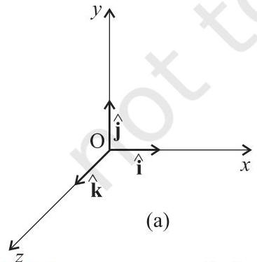 Fig. 3.9 (a) Unit vectors $\hat{\mathbf{i}}$, $\hat{\mathbf{j}}$ and $\hat{\mathbf{k}}$ lie along the $x$--, $y$--, and $z$-axes. (b) A vector $\mathbf{A}$ is resolved into its components $A_{x}$ and $A_{y}$ along $x$--, and $y$-axes. (c) $\mathbf{A}{1}$ and $\mathbf{A}{2}$ expressed in terms of $\hat{\mathbf{i}}$ and $\hat{\mathbf{j}}$.
 (b)
(b)
 (c)
(c)
MOTION IN A PLANE
Hitherto, our discussion has focused on a vector confined to an $x-y$ plane. Nevertheless, this identical methodology is applicable for decomposing a general vector $\mathbf{A}$ into three constituent components along the $x$-axis, $y$-axis, and $z$-axis within a three-dimensional space. If $\alpha$, $\beta$, and $\gamma$ denote the angles* subtended between $\mathbf{A}$ and the $x$-, $y$-, and $z$-axes, respectively [refer to Fig. 3.9(d)], then we establish:
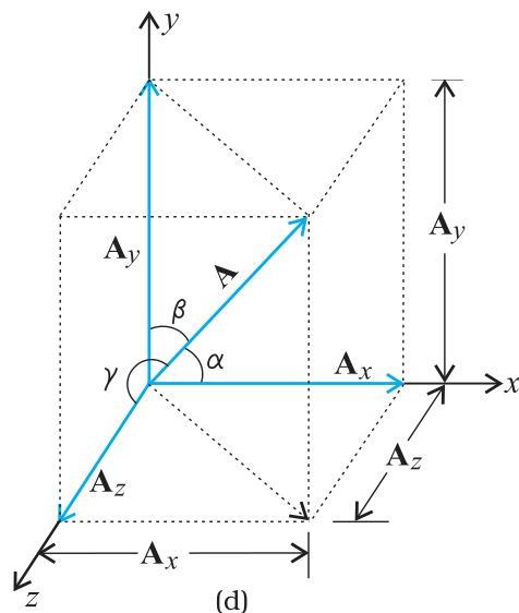 Fig. 3.9 (d) A vector $\mathbf{A}$ resolved into components along $x$-, $y$-, and $z$-axes
$\mathbf{A}{\mathbf{x}} = \mathbf{A}\cos \alpha ,\mathbf{A}{\mathbf{y}} = \mathbf{A}\cos \beta ,\mathbf{A}_{\mathbf{z}} = \mathbf{A}\cos \gamma$ (3.16a) More broadly, a vector can be expressed as:
$ \mathbf {A} = A _ {x} \hat {\mathbf {i}} + A _ {y} \hat {\mathbf {j}} + A _ {z} \hat {\mathbf {k}} \tag {3.16b} $
The magnitude of vector $\mathbf{A}$ is determined by:
$ A = \sqrt {A _ {x} ^ {2} + A _ {y} ^ {2} + A _ {z} ^ {2}} \tag {3.16c} $
A position vector $\mathbf{r}$ may be formulated as:
$ \mathbf {r} = x \hat {\mathbf {i}} + y \hat {\mathbf {j}} + z \hat {\mathbf {k}} \tag {3.17} $
Here, $x, y$, and $z$ denote the respective scalar components of $\mathbf{r}$ along the $x$-, $y$-, and $z$-axes.
3.6 VECTOR ADDITION - ANALYTICAL METHOD
While the graphical approach for vector addition offers an intuitive visualization of vectors and their resultant, it often involves laborious procedures and yields limited precision. A more straightforward and typically more accurate method involves summing vectors by combining their individual components. Consider two vectors, $\mathbf{A}$ and $\mathbf{B}$, situated within the $x-y$ plane, defined by their respective components $A_x, A_y$ and $B_x, B_y$:
$ \mathbf {A} = A _ {x} \hat {\mathbf {i}} + A _ {y} \hat {\mathbf {j}} \tag {3.18} $
$ \mathbf {B} = B _ {x} \hat {\mathbf {i}} + B _ {y} \hat {\mathbf {j}} $
If $\mathbf{R}$ represents their sum, then we have:
$ \begin{array}{l} \mathbf {R} = \mathbf {A} + \mathbf {B} \ = \left(A _ {x} \hat {\mathbf {i}} + A _ {y} \hat {\mathbf {j}}\right) + \left(B _ {x} \hat {\mathbf {i}} + B _ {y} \hat {\mathbf {j}}\right) \tag {3.19a} \ \end{array} $
Given that vectors adhere to both commutative and associative principles, the terms in Equation (3.19a) can be rearranged and grouped for convenience, yielding:
$ \mathbf {R} = \left(A _ {x} + B _ {x}\right) \hat {\mathbf {i}} + \left(A _ {y} + B _ {y}\right) \hat {\mathbf {j}} \tag {3.19b} $
$ \operatorname {S i n c e} \mathbf {R} = R _ {x} \hat {\mathbf {i}} + R _ {y} \hat {\mathbf {j}} \tag {3.20} $
Consequently, we find that $R_x = A_x + B_x$ and $R_y = A_y + B_y$ (3.21).
Therefore, each component of the resultant vector $\mathbf{R}$ is obtained by summing the corresponding components of vectors $\mathbf{A}$ and $\mathbf{B}$.
Extending this to three dimensions, we observe:
$ \begin{array}{l} \mathbf {A} = A _ {x} \hat {\mathbf {i}} + A _ {y} \hat {\mathbf {j}} + A _ {z} \hat {\mathbf {k}} \ \mathbf {B} = B _ {x} \hat {\mathbf {i}} + B _ {y} \hat {\mathbf {j}} + B _ {z} \hat {\mathbf {k}} \ \mathbf {R} = \mathbf {A} + \mathbf {B} = R _ {x} \hat {\mathbf {i}} + R _ {y} \hat {\mathbf {j}} + R _ {z} \hat {\mathbf {k}} \ \end{array} $
where $R_x = A_x + B_x$,
$ \begin{array}{l} R _ {y} = A _ {y} + B _ {y} \ R _ {z} = A _ {z} + B _ {z} \tag {3.22} \ \end{array} $
This methodology is extensible to the summation and subtraction of an arbitrary number of vectors. For instance, if vectors $\mathbf{a}$, $\mathbf{b}$, and $\mathbf{c}$ are specified as:
$ \begin{array}{l} \mathbf {a} = a _ {x} \hat {\mathbf {i}} + a _ {y} \hat {\mathbf {j}} + a _ {z} \hat {\mathbf {k}} \ \mathbf {b} = b _ {x} \hat {\mathbf {i}} + b _ {y} \hat {\mathbf {j}} + b _ {z} \hat {\mathbf {k}} \ \mathbf {c} = c _ {x} \hat {\mathbf {i}} + c _ {y} \hat {\mathbf {j}} + c _ {z} \hat {\mathbf {k}} \tag {3.23a} \ \end{array} $
Consequently, the vector $\mathbf{T}$, defined as the sum $\mathbf{a} + \mathbf{b} - \mathbf{c}$, possesses the following corresponding components:
$ \begin{array}{l} T _ {x} = a _ {x} + b _ {x} - c _ {x} \ T _ {y} = a _ {y} + b _ {y} - c _ {y} \tag {3.23b} \ T _ {z} = a _ {z} + b _ {z} - c _ {z}. \ \end{array} $
Example 3.2 Determine the magnitude and directional orientation of the resultant vector formed by two vectors, $\mathbf{A}$ and $\mathbf{B}$, expressed as functions of their individual magnitudes and the angle $\theta$ separating them.
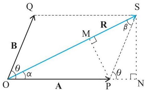 Fig. 3.10
Answer Consider two vectors, $\mathbf{A}$ and $\mathbf{B}$, depicted by segments OP and OQ respectively, forming an angle $\theta$ as shown in Fig. 3.10. Applying the parallelogram method for vector summation, the segment OS then symbolizes the resultant vector $\mathbf{R}$:
$ \mathbf {R} = \mathbf {A} + \mathbf {B} $
A perpendicular, $SN$, is drawn from $S$ to the line containing $OP$, and similarly, $PM$ is perpendicular to $OS$.
Based on the geometric configuration illustrated in the figure,
$ O S ^ {2} = O N ^ {2} + S N ^ {2} $
However, the length $ON$ can be expressed as the sum of $OP$ and $PN$, which equates to $A + B\cos \theta$
$ S N = B \sin \theta $
$ O S ^ {2} = (A + B \cos \theta) ^ {2} + (B \sin \theta) ^ {2} $
This simplifies to $R^2 = A^2 + B^2 + 2AB\cos \theta$
$ R = \sqrt {A ^ {2} + B ^ {2} + 2 A B \cos \theta} \tag {3.24a} $
Within triangle OSN, the segment $SN$ is given by $OS\sin \alpha$, which is equivalent to $R\sin \alpha$. Concurrently, in triangle PSN, $SN$ is expressed as $PS\sin \theta$, or $B\sin \theta$.
Consequently, the equality $R\sin \alpha = B\sin \theta$ holds.
This relation can be rearranged to $\frac{R}{\sin\theta} = \frac{B}{\sin\alpha}$ (3.24b)
Following a similar line of reasoning,
$ \mathrm {P M} = A \sin \alpha = B \sin \beta $
Which can be written as $\frac{A}{\sin\beta} = \frac{B}{\sin\alpha}$ (3.24c)
By synthesizing Equations (3.24b) and (3.24c), we arrive at:
$ \frac {R}{\sin \theta} = \frac {A}{\sin \beta} = \frac {B}{\sin \alpha} \tag {3.24d} $
From Equation (3.24d), we can deduce:
$ \sin \alpha = \frac {B}{R} \sin \theta \tag {3.24e} $
Here, the value of $R$ is determined by Equation (3.24a).
$ \text {o r ,} \tan \alpha = \frac {S N}{O P + P N} = \frac {B \sin \theta}{A + B \cos \theta} \tag {3.24f} $
Equation (3.24a) quantifies the magnitude of the resultant vector, while Equations (3.24e) and (3.24f) specify its directional orientation. It is noteworthy that Equation (3.24a) corresponds to the Law of Cosines, and Equation (3.24d) represents the Law of Sines.
Example 3.3 A motorboat proceeds northward at a speed of $25\mathrm{km / h}$, concurrent with a water current flowing at $10\mathrm{km / h}$ in a direction $60^{\circ}$ east of south. Determine the boat's resultant velocity.
Answer Figure 3.11 illustrates the vector $\mathbf{v}{\mathrm{b}}$, which denotes the motorboat's velocity, and the vector $\mathbf{v}{\mathrm{c}}$, representing the water current, aligned with their respective directions as outlined in the problem statement. Applying the parallelogram method for vector summation, the resultant vector $\mathbf{R}$ is derived, pointing in the direction indicated in the diagram.
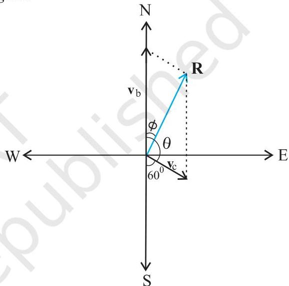 Fig. 3.11
The magnitude of $\mathbf{R}$ can be determined through the application of the Law of Cosines:
$ \begin{array}{l} R = \sqrt {v _ {\mathrm {b}} ^ {2} + v _ {\mathrm {c}} ^ {2} + 2 v _ {\mathrm {b}} v _ {\mathrm {c}} \cos 1 2 0 ^ {\circ}} \ = \sqrt {2 5 ^ {2} + 1 0 ^ {2} + 2 \times 2 5 \times 1 0 (- 1 / 2)} \cong 2 2 \mathrm {k m / h} \ \end{array} $
The direction can be ascertained by employing the Law of Sines:
$ \begin{array}{l} \frac {R}{\sin \theta} = \frac {v _ {c}}{\sin \phi} \text { or,} \sin \phi = \frac {v _ {c}}{R} \sin \theta \ = \frac {1 0 \times \sin 1 2 0 ^ {\circ}}{2 1 . 8} = \frac {1 0 \sqrt {3}}{2 \times 2 1 . 8} \cong 0. 3 9 7 \ \phi \cong 2 3. 4 ^ {\circ} \ \end{array} $
3.7 MOTION IN A PLANE
This section will elucidate the methodology for characterizing two-dimensional motion utilizing vector quantities.
3.7.1 Position Vector and Displacement
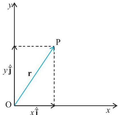
Within an $x-y$ coordinate system, the position vector $\mathbf{r}$ defining the location of a particle $\mathrm{P}$ in a two-dimensional plane, relative to the origin (as depicted in Fig. 3.12), is mathematically expressed as:
$ \mathbf {r} = x \hat {\mathbf {i}} + y \hat {\mathbf {j}} $
In this formulation, $x$ and $y$ represent the orthogonal components of $\mathbf{r}$ projected onto the $x$-axis and $y$-axis, respectively, effectively serving as the object's spatial coordinates.
 (a)
(a)
 (b)
(b)
 (a)
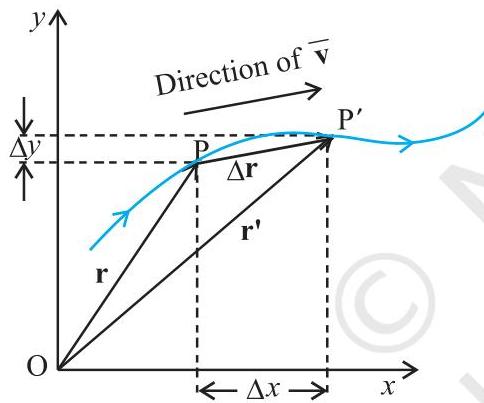
Fig. 3.12 (a) Position vector $\mathbf{r}$ . (b) Displacement $\Delta \mathbf{r}$ and average velocity $\mathbf{v}$ of a particle.
(a)
Fig. 3.12 (a) Position vector $\mathbf{r}$ . (b) Displacement $\Delta \mathbf{r}$ and average velocity $\mathbf{v}$ of a particle.
 (b)
(b)
Consider a particle traversing the trajectory delineated by the bold curve, occupying position $\mathrm{P}$ at an initial time $t$ and subsequently position $\mathrm{P}'$ at a later time $t'$ [refer to Fig. 3.12(b)]. In this scenario, the displacement is defined as:
$ \Delta \mathbf {r} = \mathbf {r} ^ {\prime} - \mathbf {r} \tag {3.25} $
This displacement vector points from the initial position $\mathrm{P}$ to the final position $\mathrm{P}'$.
Equation (3.25) can be expressed in its component form as follows:
$ \begin{array}{l} \Delta \mathbf {r} = \left(x ^ {\prime} \hat {\mathbf {i}} + y ^ {\prime} \hat {\mathbf {j}}\right) - \left(x \hat {\mathbf {i}} + y \hat {\mathbf {j}}\right) \ = \hat {\mathbf {i}} \Delta x + \hat {\mathbf {j}} \Delta y \ \end{array} $
Here, $\Delta x$ denotes the change in the $x$-coordinate, calculated as $x' - x$, and $\Delta y$ signifies the change in the $y$-coordinate, given by $y' - y$ (3.26).
Velocity
An object's average velocity, denoted as $\left(\overline{\mathbf{v}}\right)$, is defined as the quotient of its displacement and the duration over which that displacement occurs:
$ \bar {\mathbf {v}} = \frac {\Delta \mathbf {r}}{\Delta t} = \frac {\Delta x \hat {\mathbf {i}} + \Delta y \hat {\mathbf {j}}}{\Delta t} = \hat {\mathbf {i}} \frac {\Delta x}{\Delta t} + \hat {\mathbf {j}} \frac {\Delta y}{\Delta t} \tag {3.27} $
Alternatively, this can be expressed as $\overline{\mathbf{v}} = \overline{\mathbf{v}}_x\hat{\mathbf{i}} +\overline{\mathbf{v}}_y\hat{\mathbf{j}}$.
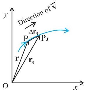
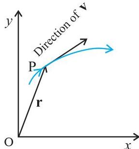
Given the definition $\overline{\mathbf{v}} = \frac{\Delta\mathbf{r}}{\Delta t}$, it follows that the average velocity's orientation corresponds directly with that of the displacement vector $\Delta \mathbf{r}$ (refer to Fig. 3.12). The instantaneous velocity, commonly referred to simply as velocity, is determined by the average velocity's limiting value as the corresponding time interval approaches zero:
$ \bar {\mathbf {v}} = \lim _ {\Delta t \rightarrow 0} \frac {\Delta \mathbf {r}}{\Delta t} = \frac {\mathrm {d} \mathbf {r}}{\mathrm {d} t} \tag {3.28} $
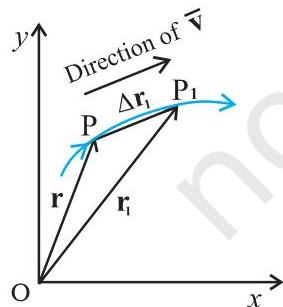
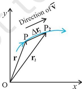
Figure 3.13(a) through (d) provides a clear illustration of the conceptual basis for this limiting process. Within these diagrams, the trajectory of an object is depicted by the bold line; at a specific time $t$, the object is located at point $\mathrm{P}$. Points $\mathrm{P}_1$, $\mathrm{P}_2$, and $\mathrm{P}_3$ denote the object's positions after elapsed time intervals of $\Delta t_1$, $\Delta t_2$, and $\Delta t_3$, respectively. The displacements corresponding to these intervals are $\Delta \mathbf{r}_1$, $\Delta \mathbf{r}_2$, and $\Delta \mathbf{r}_3$.
 (c)
(c)
 (d)
(d)
 Fig. 3.13 As the time interval $\Delta t$ approaches zero, the average velocity approaches the velocity $\mathbf{v}$ . The direction of $\overline{\mathbf{v}}$ is parallel to the line tangent to the path.
The average velocity $\overline{\mathbf{v}}
YoLearn.AI is India's #1 AI tutoring platform for Class 1 to 12, JEE, and NEET preparation.
Students talk to expert AI tutors in real time through live voice calls, solve doubts instantly
on an interactive sketch board, and practice with mock tests, flashcards, quizzes, and slide decks.
Learn from top educators including DC Pandey and other verified teachers who create AI avatars of themselves.
Unlike text-only chatbots, YoLearn.AI lets you speak naturally to your AI tutor — just like a real
one-on-one session. Get step-by-step explanations for Physics, Chemistry, Maths, and Biology
for board exams, JEE Main, JEE Advanced, and NEET.
Prepare for JEE 2026, NEET 2026, and CBSE board exams with personalized mock tests, AI-generated
quizzes, and flashcard makers. Build daily study habits with an AI study buddy designed for Indian students.
Whether you need a Class 10 CBSE tutor, Class 12 board exam help, or full JEE and NEET coaching online,
YoLearn.AI adapts to your grade, syllabus, and learning pace. Start free today on web, iOS, and Android.
Personal 1:1 AI Tutor for CBSE, JEE & NEET Students
Live voice tutoring and doubt solving
Mock tests, flashcards, and exam prep
For school, JEE, and NEET
The vector $\mathbf{v}$ can be represented using its component form as follows:
$ \begin{array}{l} \mathbf{v} = \frac{\mathrm{d} \mathbf{r}}{\mathrm{d} t} \ = \lim_{\Delta t \rightarrow 0} \left(\frac{\Delta x}{\Delta t} \hat{\mathbf{i}} + \frac{\Delta y}{\Delta t} \hat{\mathbf{j}}\right) \tag{3.29} \ = \hat{\mathbf{i}} \lim_{\Delta t \rightarrow 0} \frac{\Delta x}{\Delta t} + \hat{\mathbf{j}} \lim_{\Delta t \rightarrow 0} \frac{\Delta y}{\Delta t} \end{array} $
Alternatively, the velocity vector $\mathbf{v}$ can be expressed as: $ \mathbf{v} = \hat{\mathbf{i}} \frac{\mathrm{d} x}{\mathrm{d} t} + \hat{\mathbf{j}} \frac{\mathrm{d} y}{\mathrm{d} t} = v_{x} \hat{\mathbf{i}} + v_{y} \hat{\mathbf{j}}. $ Here, the components $v_{x}$ and $v_{y}$ are defined as $v_{x} = \frac{\mathrm{d} x}{\mathrm{d} t}$ and $v_{y} = \frac{\mathrm{d} y}{\mathrm{d} t}$ respectively. \tag{3.30a}
Consequently, if the temporal dependencies of the coordinates $x$ and $y$ are established, these equations enable the determination of $v_{x}$ and $v_{y}$.
The scalar magnitude of $\mathbf{v}$ is subsequently calculated as:
$ v = \sqrt{v_{x}^{2} + v_{y}^{2}} \tag{3.30b} $
Furthermore, the orientation of $\mathbf{v}$ is specified by the angle $\theta$:
$ \tan \theta = \frac{v_{y}}{v_{x}}, \quad \theta = \tan^{-1} \left(\frac{v_{y}}{v_{x}}\right) \tag{3.30c} $
The components $v_{x}, v_{y}$, and the angle $\theta$ are visually represented in Fig. 3.14, corresponding to a velocity vector $\mathbf{v}$ at a specific point $\mathbf{p}$.
Acceleration
For an object traversing the $x-y$ plane over a time interval $\Delta t$, the mean acceleration $\overline{\mathbf{a}}$ is defined as the ratio of the alteration in its velocity to that time interval:
$ \overline{\mathbf{a}} = \frac{\Delta \mathbf{v}}{\Delta t} = \frac{\Delta \left(v_{x} \hat{\mathbf{i}} + v_{y} \hat{\mathbf{j}}\right)}{\Delta t} = \frac{\Delta v_{x}}{\Delta t} \hat{\mathbf{i}} + \frac{\Delta v_{y}}{\Delta t} \hat{\mathbf{j}} \tag{3.31a} $
Expressed differently,
$ \overline{\mathbf{a}} = a_{x} \hat{\mathbf{i}} + a_{y} \hat{\mathbf{j}}. \tag{3.31b} $
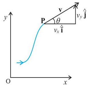 Fig. 3.14 The components $v_{x}$ and $v_{y}$ of velocity $\mathbf{v}$ and the angle $\theta$ it makes with $x$-axis. Note that $v_{x} = v \cos \theta$, $v_{y} = v \sin \theta$.
The instantaneous acceleration, denoted as $\mathbf{a}$, is derived as the limit of the average acceleration as the time interval approaches zero:
$ \mathbf{a} = \lim_{\Delta t \rightarrow 0} \frac{\Delta \mathbf{v}}{\Delta t} \tag{3.32a} $
Given that $\Delta \mathbf{v}$ can be expressed as $\Delta v_{x} \hat{\mathbf{i}} + \Delta v_{y} \hat{\mathbf{j}}$, the instantaneous acceleration becomes:
$ \mathbf{a} = \hat{\mathbf{i}} \lim_{\Delta t \rightarrow 0} \frac{\Delta v_{x}}{\Delta t} + \hat{\mathbf{j}} \lim_{\Delta t \rightarrow 0} \frac{\Delta v_{y}}{\Delta t} $
This can be concisely written as:
$ \mathbf{a} = a_{x} \hat{\mathbf{i}} + a_{y} \hat{\mathbf{j}} \tag{3.32b} $
where the components $a_{x}$ and $a_{y}$ are defined by $a_{x} = \frac{\mathrm{d}v_{x}}{\mathrm{d}t}$ and $a_{y} = \frac{\mathrm{d}v_{y}}{\mathrm{d}t}$. \tag{3.32c}*
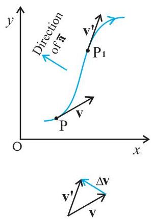
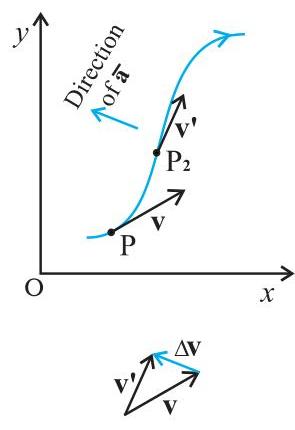
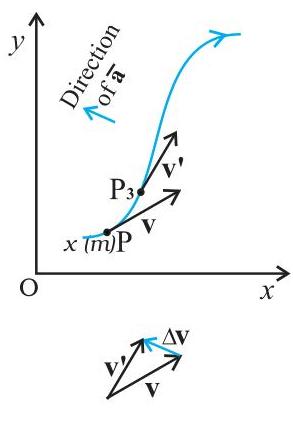
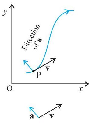
Similar to the methodology employed for velocity, the limiting process fundamental to the definition of acceleration can be elucidated graphically by examining the trajectory of the object's motion. This visualization is presented in Figs. 3.15(a) through (d). Point P signifies the object's position at time $t$, with $P_{1}, P_{2}, P_{3}$ denoting subsequent positions after respective time increments $\Delta t_{1}, \Delta t_{2}, \Delta t_{3}$, where $\Delta t_{1} > \Delta t_{2} > \Delta t_{3}$. The velocity vectors corresponding to points $P, P_{1}, P_{2}, P_{3}$ are also depicted in Figs. 3.15 (a), (b), and (c). For each distinct $\Delta t$, the change in velocity, $\Delta \mathbf{v}$, is ascertained through the application of the triangle law for vector addition. By definition, the average acceleration's direction coincides with that of $\Delta \mathbf{v}$. It is observable that as $\Delta t$ diminishes, the orientation of $\Delta \mathbf{v}$ undergoes alteration, and consequently, the direction of the acceleration vector changes. Ultimately, as $\Delta t$ approaches zero [Fig. 3.15(d)], the average acceleration converges to the instantaneous acceleration, assuming the direction illustrated.
MOTION IN A PLANE
 (a)
(a)
 (b)
(b)
 (c)
Fig. 3.15 Depicts the average acceleration across three distinct time intervals: (a) $\Delta t_1$, (b) $\Delta t_2$, and (c) $\Delta t_3$, where $(\Delta t_1 > \Delta t_2 > \Delta t_3)$. (d) Illustrates how, as the time interval $\Delta t$ approaches zero, the average acceleration converges to the instantaneous acceleration.
(c)
Fig. 3.15 Depicts the average acceleration across three distinct time intervals: (a) $\Delta t_1$, (b) $\Delta t_2$, and (c) $\Delta t_3$, where $(\Delta t_1 > \Delta t_2 > \Delta t_3)$. (d) Illustrates how, as the time interval $\Delta t$ approaches zero, the average acceleration converges to the instantaneous acceleration.
 (d)
(d)
It is important to recognize that for one-dimensional motion, an object's velocity and acceleration vectors invariably align along a single straight axis, either pointing in the same direction or in diametrically opposite directions. In contrast, when considering motion in two or three dimensions, the velocity and acceleration vectors can exhibit any angular separation ranging from $0^{\circ}$ to $180^{\circ}$.
Example 3.4 Consider a particle whose position is described by the vector function:
$ \mathbf {r} = 3. 0 t \hat {\mathbf {i}} + 2. 0 t ^ {2} \hat {\mathbf {j}} + 5. 0 \hat {\mathbf {k}} $
Here, $t$ is measured in seconds, and the numerical coefficients are dimensionally consistent such that $\mathbf{r}$ is expressed in meters. (a) Determine the particle's velocity vector, $\mathbf{v}(t)$, and acceleration vector, $\mathbf{a}(t)$, as functions of time. (b) Calculate the magnitude and specify the direction of $\mathbf{v}(t)$ at the specific instant $t = 1.0 , \text{s}$.
Answer
$ \begin{array}{l} \mathbf {v} (t) = \frac {\mathrm {d} \mathbf {r}}{\mathrm {d} t} = \frac {\mathrm {d}}{\mathrm {d} t} \left(3. 0 t \hat {\mathbf {i}} + 2. 0 t ^ {2} \hat {\mathbf {j}} + 5. 0 \hat {\mathbf {k}}\right) \ = 3. 0 \hat {\mathbf {i}} + 4. 0 t \hat {\mathbf {j}} \ \end{array} $
$ \mathbf {a} (t) = \frac {\mathrm {d} \mathbf {v}}{\mathrm {d} t} = + 4. 0 \hat {\mathbf {j}} $
$ a = 4. 0 \mathrm {m} \mathrm {s} ^ {- 2} \text { along } y - \text { direction} $
At $t = 1.0\mathrm{s}$, the velocity vector is $\mathbf{v} = 3.0\hat{\mathbf{i}} +4.0\hat{\mathbf{j}}$.
Its magnitude is $v = \sqrt{3^2 + 4^2} = 5.0 , \text{m s}^{-1}$, and its direction is given by
$ \theta = \tan^ {- 1} \left(\frac {v _ {y}}{v _ {x}}\right) = \tan^ {- 1} \left(\frac {4}{3}\right) \cong 5 3 ^ {\circ} \text { with } x \text {- a x i s}. $
3.8 MOTION IN A PLANE WITH CONSTANT ACCELERATION
Consider an object traversing the $x-y$ plane under the influence of a constant acceleration, denoted by $\mathbf{a}$. Given this constancy, the average acceleration over any time interval will precisely correspond to this fixed value. If the object possesses an initial velocity $\mathbf{v}_0$ at time $t=0$, and subsequently attains a velocity $\mathbf{v}$ at a later time $t$, then, by fundamental definition,
$ \mathbf {a} = \frac {\mathbf {v} - \mathbf {v} _ {0}}{t - 0} = \frac {\mathbf {v} - \mathbf {v} _ {0}}{t} $
Or, $\mathbf{v} = \mathbf{v_0} + \mathbf{a}t$ (3.33a)
In terms of components :
$ v _ {x} = v _ {o x} + a _ {x} t $
$ v _ {y} = v _ {o y} + a _ {y} t \tag {3.33b} $
Next, our objective is to determine the temporal evolution of the position vector $\mathbf{r}$. We shall adopt an approach analogous to that employed for one-dimensional motion. Let $\mathbf{r}_0$ and $\mathbf{r}$ represent the position vectors of the particle at the initial moment, $t=0$, and at time $t$, respectively. Concurrently, let the corresponding velocities at these specific instants be $\mathbf{v}_0$ and $\mathbf{v}$. Over this duration $t$, the average velocity is expressed as $(\mathbf{v}_0 + \mathbf{v}) / 2$. Consequently, the displacement is obtained by multiplying this average velocity by the elapsed time interval:
$
\begin{array}{l} \mathbf{r} - \mathbf{r}_0 = \left(\frac{\mathbf{v} + \mathbf{v}_0}{2}\right) t = \left(\frac{(\mathbf{v}_0 + \mathbf{a} t) + \mathbf{v}_0}{2}\right) t \ = \mathbf{v}_0 t + \frac{1}{2} \mathbf{a} t^2 \end{array} $
$ \text{Or,} \quad \mathbf{r} = \mathbf{r}_0 + \mathbf{v}_0 t + \frac{1}{2} \mathbf{a} t^2 \tag{3.34a} $
One can readily confirm that differentiating Equation (3.34a) with respect to time, i.e., calculating $\frac{\mathrm{d}\mathbf{r}}{\mathrm{d}t}$, yields Equation (3.33a). Furthermore, this relation correctly satisfies the initial condition that $\mathbf{r} = \mathbf{r}_0$ when $t = 0$. Equation (3.34a) is also representable in its component form as:
$ x = x_0 + v_{\mathrm{ox}} t + \frac{1}{2} a_x t^2 $
$ y = y_0 + v_{\mathrm{oy}} t + \frac{1}{2} a_y t^2 \tag{3.34b} $
A direct consequence of Equation (3.34b) is the principle that motion along the $x$-direction and motion along the $y$-direction are mutually independent. In essence, planar (two-dimensional) motion can be conceptualized as the superposition of two distinct, simultaneous one-dimensional motions, each characterized by constant acceleration and occurring along orthogonal axes. This fundamental insight proves invaluable for the analytical examination of object motion in two dimensions. An analogous principle is applicable to three-dimensional scenarios. The judicious selection of mutually perpendicular directions frequently simplifies the analysis of various physical phenomena, as will become evident in our discussion of projectile motion in Section 3.9.
Example 3.5 A particle commences its motion from the origin at $t = 0$, possessing an initial velocity of $5.0 , \mathrm{km/s}$. It navigates the $x-y$ plane under the influence of a constant force, which imparts a constant acceleration of $(3.0\hat{\mathbf{i}} + 2.0\hat{\mathbf{j}}) , \mathrm{m/s^2}$. (a) Determine the $y$-coordinate of the particle at the precise moment its $x$-coordinate reaches $84 , \mathrm{m}$. (b) Calculate the speed of the particle at this particular instant.
Answer From Eq. (3.34a) for $\mathbf{r}_0 = 0$, the position of the particle is given by
$ \begin{array}{l} \mathbf{r}(t) = \mathbf{v}_0 t + \frac{1}{2} \mathbf{a} t^2 \ = 5.0 \hat{\mathbf{i}} t + (1/2) (3.0 \hat{\mathbf{i}} + 2.0 \hat{\mathbf{j}}) t^2 \end{array} $
$ = (5.0 t + 1.5 t^2) \hat{\mathbf{i}} + 1.0 t^2 \hat{\mathbf{j}} $
Therefore, $x(t) = 5.0 t + 1.5 t^2$
$ y(t) = +1.0 t^2 $
Given $x(t) = 84 , \mathrm{m}, t = ?$
$ 5.0 t + 1.5 t^2 = 84 \Rightarrow t = 6 , \mathrm{s} $
At $t = 6 , \mathrm{s}$, $y = 1.0 , (6)^2 = 36.0 , \mathrm{m}$
Now, the velocity $\mathbf{v} = \frac{\mathrm{d}\mathbf{r}}{\mathrm{d}t} = (5.0 + 3.0 t) \hat{\mathbf{i}} + 2.0 t \hat{\mathbf{j}}$
At $t = 6 , \mathrm{s}$, $\mathbf{v} = 23.0 \hat{\mathbf{i}} + 12.0 \hat{\mathbf{j}}$
speed $= |\mathbf{v}| = \sqrt{23^2 + 12^2} \cong 26 , \mathrm{m} , \mathrm{s}^{-1}$.
3.9 PROJECTILE MOTION
Building upon the concepts established in preceding sections, we now delve into the dynamics of projectile motion. A projectile is defined as any object that remains airborne subsequent to being cast or propelled. Examples include a football, a cricket ball, a baseball, or similar items. The trajectory of a projectile can be conceptualized as the amalgamation of two distinct and concurrent motion components. One component proceeds along a horizontal axis, devoid of acceleration, while the other traverses the vertical axis under the influence of constant gravitational acceleration. This fundamental principle of independence between the horizontal and vertical constituents of projectile motion was initially articulated by Galileo in his seminal work, Dialogue on the Great World Systems (1632).
For the purposes of this analysis, we will presuppose that atmospheric drag exerts an inconsequential influence on the projectile's trajectory. Let us consider a scenario where the projectile is initiated with an initial velocity $\mathbf{v}_0$, forming an angle $\theta_0$ with the horizontal $x$-axis, as depicted in Fig. 3.16.
Following the projection of the object, the sole acceleration influencing its motion is that attributed to gravity, which is oriented vertically downwards:
$ \mathbf{a} = -g \hat{\mathbf{j}} $
$ \text{Alternatively,} \quad a_x = 0, , a_y = -g \tag{3.35} $
The constituent components of the initial velocity $\mathbf{v}_0$ are expressed as:
$ \begin{array}{l} v_{\mathrm{ox}} = v_0 \cos \theta_0 \ v_{\mathrm{oy}} = v_0 \sin \theta_0 \tag{3.36} \end{array}
$
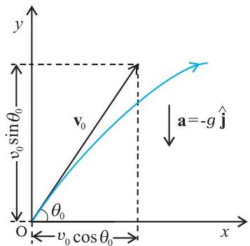 Fig 3.16 Motion of an object projected with velocity $\mathbf{v}_o$ at angle $\theta_0$ .
Assuming the initial coordinates coincide with the origin of the chosen reference frame, as illustrated in Fig. 3.16, we establish:
$ x _ {o} = 0, y _ {o} = 0 $
Consequently, Equation (3.34b) transforms into:
$ x = v _ {o x} t = \left(v _ {o} \cos \theta_ {o}\right) t $
and $y = (v_{o}\sin \theta_{o})t - (\frac{1}{2})gt^{2}$ (3.37)
The velocity components at an arbitrary time $t$ are determinable via Equation (3.33b):
$ v _ {x} = v _ {o x} = v _ {o} \cos \theta_ {o} $
$ v _ {y} = v _ {o} \sin \theta_ {o} - g t \tag {3.38} $
Equation (3.37) delineates the $x$- and $y$-coordinates defining a projectile's position at any given time $t$, expressed as functions of two primary parameters: the initial speed $v_{o}$ and the launch angle $\theta_{o}$. A significant simplification arises from the judicious selection of orthogonal $x$- and $y$-axes for analyzing projectile motion. Specifically, the $x$-component of the velocity maintains a constant magnitude throughout the trajectory, whereas only the $y$-component undergoes alteration, mirroring the behavior of an object in vertical free fall. This phenomenon is visually represented at various time points in Fig. 3.17. It is noteworthy that at the apex of its trajectory, the velocity component $v_{t}$ becomes zero; consequently,
$ \theta = \tan^ {- 1} \frac {v _ {y}}{v _ {x}} = 0 $
Equation of path of a projectile
To ascertain the trajectory's form, one can eliminate the temporal variable from the kinematic equations describing the horizontal ($x$) and vertical ($y$) components of motion, as presented in Eq. (3.37). This yields:
$ y = \left(\tan \theta_ {o}\right) x - \frac {g}{2 \left(v _ {o} \cos \theta_ {o}\right) ^ {2}} x ^ {2} \tag {3.39} $
Given that the gravitational acceleration ($g$), initial projection angle ($\theta_o$), and initial velocity magnitude ($v_o$) are invariant quantities, Equation (3.39) can be recognized as conforming to the general quadratic form $y = ax + bx^2$, where $a$ and $b$ represent constant coefficients. This mathematical structure intrinsically defines a parabola, thereby establishing that the projectile's trajectory is parabolic in nature (refer to Fig. 3.17).
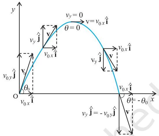 Fig. 3.17 The path of a projectile is a parabola.
Time of maximum height
To ascertain the duration required for the projectile to reach its zenith, we define this period as $t_m$. Given that the vertical component of velocity, $v_t$, is zero at this point, we can derive from Equation (3.38):
$ v _ {y} = v _ {o} \sin \theta_ {o} - g t _ {m} = 0 $
Or, $t_m = v_o \sin \theta_o / g$ (3.40a)
The aggregate duration, denoted $T_f$, for which the projectile remains airborne can be ascertained by setting the vertical displacement $y$ to zero in Equation (3.37). This yields:
$ T _ {f} = 2 \left(v _ {o} \sin \theta_ {o}\right) / g \tag {3.40b} $
The quantity $T_f$ is commonly referred to as the projectile's time of flight. It is noteworthy that $T_f = 2t_m$, a relationship consistent with the inherent symmetry characteristic of a parabolic trajectory.
Maximum height of a projectile
The apex height, denoted as $h_m$, attained by a projectile is ascertained by inserting $t = t_m$ into Equation (3.37):
$ y = h _ {m} = \left(v _ {0} \sin \theta_ {0}\right) \left(\frac {v _ {0} \sin \theta_ {0}}{g}\right) - \frac {g}{2} \left(\frac {v _ {0} \sin \theta_ {0}}{g}\right) ^ {2} $
Alternatively, the maximum height can be expressed as: $h_m = \frac{\left(v_0\sin\theta_0\right)^2}{2g}$ (3.41)
Horizontal range of a projectile
The horizontal displacement covered by a projectile, measured from its launch point $(x = y = 0)$ to the point where it returns to the initial vertical level ($y = 0$) during its trajectory, is termed the horizontal
range, $R$. This represents the total distance traversed during the projectile's time of flight, $T_f$. Consequently, the range $R$ is given by:
$ \begin{array}{l} R = \left(v_o \cos \theta_o\right) \left(T_f\right) \ = \left(v_o \cos \theta_o\right) \left(2 v_o \sin \theta_o\right) / g \end{array} $
Thus,
$ R = \frac{v_0^2 \sin 2\theta_0}{g} \tag{3.42a} $
From Equation (3.42a), it is evident that for a fixed initial projection velocity $v_o$, the maximum range $R$ is achieved when the term $\sin 2\theta_0$ reaches its peak value, which occurs when $\theta_0 = 45^\circ$.
Hence, the maximum horizontal range is determined as:
$ R_m = \frac{v_0^2}{g} \tag{3.42b} $
Example 3.6 In his seminal work, Two New Sciences, Galileo posited that "for launch angles that deviate equally above or below 45 degrees, the resulting horizontal ranges are identical." Provide a proof for this assertion.
Answer Consider a projectile initiated with an initial velocity vector $\mathbf{v}_0$ at an angle $\theta_o$ relative to the horizontal; its range is defined by:
$ R = \frac{v_0^2 \sin 2\theta_0}{g} $
Let us consider projection angles of $(45^\circ + \alpha)$ and $(45^\circ - \alpha)$. For these angles, the corresponding $2\theta_0$ values become $(90^\circ + 2\alpha)$ and $(90^\circ - 2\alpha)$, respectively. Trigonometrically, the sine of $(90^\circ + 2\alpha)$ and the sine of $(90^\circ - 2\alpha)$ are equivalent, both equaling $\cos 2\alpha$. Consequently, the horizontal ranges achieved are identical for launch angles that are symmetrically displaced by an amount $\alpha$ from $45^\circ$.
Example 3.7 A hiker situated at the precipice of a cliff, $490,\mathrm{m}$ above the terrain below, propels a stone horizontally with an initial velocity of $15,\mathrm{m,s^{-1}}$. Disregarding the effects of air resistance, determine both the duration until the stone impacts the ground and its final impact speed. (Assume $g = 9.8,\mathrm{m,s^{-2}}$).
Answer For this analysis, we establish the coordinate origin $(x=0, y=0)$ at the cliff's edge, with $t = 0$ s corresponding to the moment the stone is released. The positive $x$-axis is aligned with the initial horizontal velocity, and the positive $y$-axis points vertically upward. The horizontal and vertical components of the stone's motion can be analyzed separately. The governing equations of motion are as follows:
$ x(t) = x_o + v_{ox} t $
$ \begin{array}{l} y(t) = y_o + v_{oy} t + (1/2) a_y t^2 \ \text{Here,} \quad x_o = y_o = 0, , v_{oy} = 0, , a_y = -g = -9.8,\mathrm{m,s^{-2}}, \ \quad v_{ox} = 15,\mathrm{m,s^{-1}}. \end{array} $
The condition for the stone impacting the ground is defined by $y(t) = -490,\mathrm{m}$.
$ -490,\mathrm{m} = -(1/2)(9.8) t^2. $
Solving this yields $t = 10,\mathrm{s}$.
The constituent velocity components are $v_x = v_{ox}$ and
$ v_y = v_{oy} - g t $
Upon impact with the ground, the stone exhibits the following velocity components:
$ \begin{array}{l} v_{ox} = 15,\mathrm{m,s^{-1}} \ v_{oy} = 0 - 9.8 \cdot 10 = -98,\mathrm{m,s^{-1}} \end{array} $
Consequently, the magnitude of the stone's velocity is determined as:
$ \sqrt{v_x^2 + v_y^2} = \sqrt{15^2 + 98^2} = 99,\mathrm{m,s^{-1}} $
Example 3.8 A cricket ball is projected at an initial velocity of $28,\mathrm{m,s^{-1}}$ at an angle of 30 degrees above the horizontal plane. Determine: (a) its peak altitude, (b) the total duration for the ball to descend back to its initial elevation, and (c) the horizontal range from the launch point to where the ball lands at the same elevation.
Answer (a) The peak altitude, or maximum height, is computed using the following expression:
$ \begin{array}{l} h_m = \frac{(v_0 \sin \theta_o)^2}{2g} = \frac{(28 \sin 30^\circ)^2}{2(9.8)} ,\mathrm{m} \ = \frac{14 \times 14}{2 \times 9.8} = 10.0,\mathrm{m} \end{array} $
(b) The total flight time until the ball reaches its original height is given by:
$ \begin{array}{l} T_f = \left(2 v_o \sin \theta_o\right) / g = (2 \cdot 28 \sin 30^\circ) / 9.8 \ = 28 / 9.8,\mathrm{s} = 2.9,\mathrm{s} \end{array} $
(c) The horizontal distance covered from the point of projection to the point where the ball returns to the same level is calculated as:
$ R = \frac{(v_o^2 \sin 2\theta_o)}{g} = \frac{28 \times 28 \times \sin 60^\circ}{9.8} = 69,\mathrm{m} $
3.10 UNIFORM CIRCULAR MOTION
When an object traverses a circular trajectory at a consistent speed, this type of movement is termed uniform circular motion. The descriptor "uniform" signifies that the object's speed remains constant throughout its entire path. Consider an object moving at a steady speed $v$ along a circle of radius $R$, as illustrated in Fig. 3.18. Given that the object's velocity continuously alters its direction, the object must be undergoing acceleration. Our objective is to determine both the magnitude and the directional aspect of this acceleration.
 (a)
(a)
 (b)
(b)
 (c)
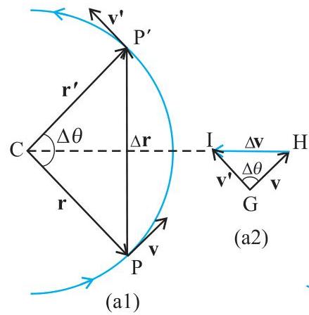
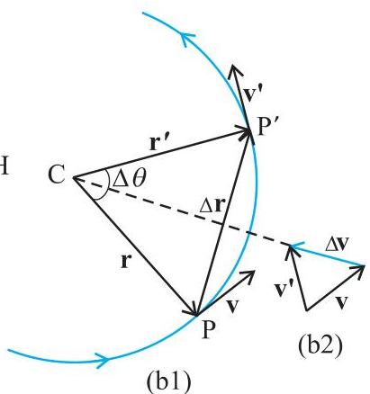
Fig. 3.18 Velocity and acceleration of an object in uniform circular motion. The time interval $\Delta t$ decreases from (a) to (c) where it is zero. The acceleration is directed, at each point of the path, towards the centre of the circle.
(c)
Fig. 3.18 Velocity and acceleration of an object in uniform circular motion. The time interval $\Delta t$ decreases from (a) to (c) where it is zero. The acceleration is directed, at each point of the path, towards the centre of the circle.
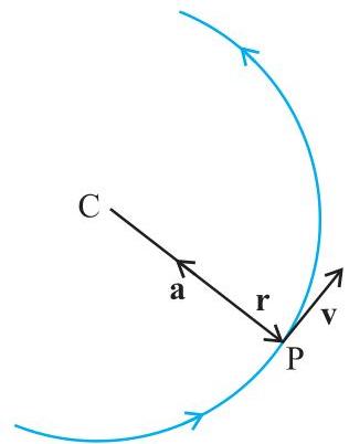
Let $\mathbf{r}$ and $\mathbf{r}'$ denote the position vectors, and $\mathbf{v}$ and $\mathbf{v}'$ represent the velocities of the object at points $P$ and $P'$ respectively, as depicted in Fig. 3.18(a). By definition, the velocity at any given point is oriented tangentially to the path at that point, aligned with the direction of motion. The velocity vectors $\mathbf{v}$ and $\mathbf{v}'$ are displayed in Fig. 3.18(a1). The change in velocity, $\Delta \mathbf{v}$, is derived in Fig. 3.18(a2) through the triangle law of vector addition. Due to the circular nature of the path, $\mathbf{v}$ is perpendicular to $\mathbf{r}$, and similarly, $\mathbf{v}'$ is perpendicular to $\mathbf{r}'$. Consequently, $\Delta \mathbf{v}$ is perpendicular to $\Delta \mathbf{r}$. Since the average acceleration is directed along $\Delta \mathbf{v}$ (i.e., $\overline{\mathbf{a}} = \frac{\Delta\mathbf{v}}{\Delta t}$), it follows that the average acceleration $\overline{\mathbf{a}}$ is perpendicular to $\Delta \mathbf{r}$. If we position $\Delta \mathbf{v}$ along the line bisecting the angle between $\mathbf{r}$ and $\mathbf{r}'$, it becomes evident that its direction points towards the center of the circle. Figure 3.18(b) illustrates these same quantities for a reduced time interval. Here, $\Delta \mathbf{v}$, and thus $\overline{\mathbf{a}}$, is once again oriented towards the center. In Fig. 3.18(c), as $\Delta t \to 0$, the average acceleration converges to the instantaneous acceleration, which is directed towards the center*. Therefore, we ascertain that the acceleration experienced by an object in uniform circular motion consistently points towards the center of the circle. We shall now proceed to determine the magnitude of this acceleration.
The magnitude of $\mathbf{a}$ is, by definition, given by
$ | \mathbf {a} | = \lim_{\Delta t \to 0} \frac {| \Delta \mathbf {v} |}{\Delta t} $
Let $\Delta \theta$ represent the angle between the position vectors $\mathbf{r}$ and $\mathbf{r}^{\prime}$. Because the velocity vectors $\mathbf{v}$ and $\mathbf{v}^{\prime}$ are always perpendicular to their respective position vectors, the angle between the velocity vectors is also $\Delta \theta$. Hence, the triangle CPP' formed by the position vectors and the triangle GHI formed by the velocity vectors $\mathbf{v},\mathbf{v}^{\prime}$ and $\Delta \mathbf{v}$ are geometrically similar (Fig. 3.18a). This similarity implies that the ratio of the base-length to the side-length for one triangle is equivalent to that of the other triangle. That is :
$ \frac {\left| \Delta \mathbf {v} \right|}{v} = \frac {\left| \Delta \mathbf {r} \right|}{R} $
Or,
$ | \Delta \mathbf {v} | = v \frac {| \Delta \mathbf {r} |}{R} $
Therefore,
$ | \mathbf {a} | = \lim _ {\Delta t \rightarrow 0} \frac {| \Delta \mathbf {v} |}{\Delta t} = \lim _ {\Delta t \rightarrow 0} \frac {v | \Delta \mathbf {r} |}{R \Delta t} = \frac {v}{R} \lim _ {\Delta t \rightarrow 0} \frac {| \Delta \mathbf {r} |}{\Delta t} $
When the time interval $\Delta t$ is infinitesimally small, the corresponding angular displacement $\Delta \theta$ is also negligible. In such a scenario, the arc length $PP'$ can be considered an accurate approximation of the magnitude of the displacement vector $|\Delta \mathbf{r}|$ :
$ \left| \Delta \mathbf {r} \right| \cong v \Delta t $
$ \frac {\left| \Delta \mathbf {r} \right|}{\Delta t} \cong v $
Or, $\lim_{\Delta t\to 0}\frac{|\Delta\mathbf{r}|}{\Delta t} = v$
Therefore, the centripetal acceleration $a_{c}$ is :
$
a _ {c} = \left(\frac {v}{R}\right) v = v ^ {2} / R \tag {3.43} $
Consequently, for an object undergoing circular motion at a constant speed $\nu$ along a path of radius $R$, its acceleration possesses a magnitude of $\nu^2 / R$ and is perpetually oriented towards the central point of the circular trajectory. This characteristic directionality is the basis for its designation as centripetal acceleration, a nomenclature introduced by Newton. While the Dutch physicist Christiaan Huygens (1629-1695) provided the initial comprehensive exposition of centripetal acceleration in 1673, it is plausible that Newton had conceptualized it prior to this publication. The etymology of "centripetal" can be traced to a Greek word signifying 'centre-seeking'. Given that both the speed $\nu$ and the radius $R$ remain invariant, the scalar value (magnitude) of the centripetal acceleration is likewise constant. Nevertheless, its directional component undergoes continuous alteration, consistently orienting itself towards the circle's center. Consequently, centripetal acceleration does not qualify as a constant vector quantity.
An alternative framework exists for characterizing the velocity and acceleration pertinent to an object undergoing uniform circular motion. When the object traverses from point $\mathbf{P}$ to $\mathbf{P}'$ over a time interval $\Delta t (= t' - t)$, the radial line segment CP (refer to Fig. 3.18) sweeps through an angle denoted as $\Delta \theta$. This $\Delta \theta$ is identified as the angular displacement. We formally define angular speed, symbolized by $\omega$ (the Greek letter omega), as the rate at which angular displacement changes with respect to time:
$ \omega = \frac {\Delta \theta}{\Delta t} \tag {3.44} $
Subsequently, if $\Delta s$ represents the linear distance covered by the object during the duration $\Delta t$ (meaning $PP'$ corresponds to $\Delta s$), then we can state:
$ v = \frac {\Delta s}{\Delta t} $
However, given the relationship $\Delta s = R\Delta \theta$, it follows that:
$ v = R \frac {\Delta \theta}{\Delta t} = R \omega $
$ v = R \omega \tag {3.45} $
It is also possible to articulate the centripetal acceleration $a_{c}$ using the angular speed as a parameter:
$ a _ {c} = \frac {v ^ {2}}{R} = \frac {\omega^ {2} R ^ {2}}{R} = \omega^ {2} R $
$ a _ {c} = \omega^ {2} R \tag {3.46} $
The duration required for an object to complete a single full revolution is termed its time period, $T$. Conversely, the frequency, $\nu (= 1 / T)$, represents the count of revolutions executed per second. During the span of one time period, the linear distance covered by the object is precisely $s = 2\pi R$. Consequently, the linear speed $\nu$ can be expressed as:
$ \nu = 2\pi R / T = 2\pi R\nu \tag{3.47} $
When considering the frequency $\nu$, the following relationships hold:
$ \omega = 2 \pi \nu $
$ \nu = 2 \pi R \nu $
$ a _ {c} = 4 \pi^ {2} v ^ {2} R \tag {3.48} $
Example 3.9 An insect confined within a circular groove of radius $12 , \text{cm}$ traverses the groove steadily, completing 7 revolutions over a period of $100 , \text{s}$. (a) Determine the angular speed and the linear speed of this motion. (b) Is the acceleration vector constant? What is its magnitude?
Answer This scenario exemplifies uniform circular motion. Here, the radius $R = 12 , \text{cm}$. The angular speed, $\omega$, is calculated as:
$ \omega = 2 \pi / T = 2 \pi \quad 7 / 100 = 0.44 , \text{rad/s} $
The linear speed, $\nu$, is:
$ \nu = \omega R = 0.44 , \text{s}^{-1} \quad 12 , \text{cm} = 5.3 , \text{cm} , \text{s}^{-1} $
The velocity vector, $\mathbf{v}$, is directed along the tangent to the circle at every instantaneous point. The acceleration, conversely, is oriented towards the center of the circle. Given that this direction changes continuously, the acceleration vector in this context is not a constant. Nevertheless, the magnitude of the acceleration remains constant:
$ \begin{array}{l} a = \omega^ {2} R = (0.44 , \text{s}^{-1}) ^ {2} (12 , \text{cm}) \ = 2.3 , \text{cm} , \text{s}^{-2} \ \end{array}
$
SUMMARY
Quantities that are solely characterized by their magnitude are known as scalar quantities. Illustrative instances include distance, speed, mass, and temperature.
Vector quantities possess both magnitude and direction. Displacement, velocity, and acceleration serve as examples. These quantities adhere to specific principles of vector algebra.
When a vector $\mathbf{A}$ is scaled by a real number $\lambda$, the outcome is another vector. The magnitude of this resulting vector is $\lambda$ times the magnitude of $\mathbf{A}$, and its direction either aligns with or opposes that of $\mathbf{A}$, contingent upon $\lambda$ being positive or negative, respectively.
The graphical summation of two vectors, $\mathbf{A}$ and $\mathbf{B}$, can be accomplished through either the head-to-tail technique or the parallelogram method.
The operation of vector addition exhibits commutativity:
$ \mathbf{A} + \mathbf{B} = \mathbf{B} + \mathbf{A} $
Furthermore, it adheres to the associative principle:
$ (\mathbf{A} + \mathbf{B}) + \mathbf{C} = \mathbf{A} + (\mathbf{B} + \mathbf{C}) $
A null vector, also termed a zero vector, is characterized by having a magnitude of zero. Given its zero magnitude, the specification of its direction is unnecessary. Its properties include:
$ \mathbf{A} + \mathbf{0} = \mathbf{A} $
$ \lambda \mathbf{0} = \mathbf{0} $
$ 0 \mathbf{A} = \mathbf{0} $
Vector subtraction, specifically the operation of subtracting $\mathbf{B}$ from $\mathbf{A}$, is formally defined as the addition of $\mathbf{A}$ and the negative of $\mathbf{B}$:
$ \mathbf{A} - \mathbf{B} = \mathbf{A} + (-\mathbf{B}) $
It is possible to decompose a vector $\mathbf{A}$ into components aligned with two specified vectors, $\mathbf{a}$ and $\mathbf{b}$, provided they reside within the same plane:
$ \mathbf{A} = \lambda \mathbf{a} + \mu \mathbf{b} $
Here, $\lambda$ and $\mu$ denote real numbers.
A unit vector corresponding to a vector $\mathbf{A}$ possesses a magnitude of 1 and shares the same direction as $\mathbf{A}$:
$ \hat{\mathbf{n}} = \frac{\mathbf{A}}{|\mathbf{A}|} $
In a right-handed coordinate system, the unit vectors $\hat{\mathbf{i}}, \hat{\mathbf{j}}, \hat{\mathbf{k}}$ each have a magnitude of one and are directed along the positive $x$, $y$, and $z$-axes, respectively.
A vector $\mathbf{A}$ is representable as:
$ \mathbf{A} = A_x \hat{\mathbf{i}} + A_y \hat{\mathbf{j}} $
Here, $A_x$ and $A_y$ signify its components along the $x$ and $y$-axes, respectively. Should the vector $\mathbf{A}$ subtend an angle $\theta$ with the $x$-axis, then $A_x$ is given by $A \cos \theta$, $A_y$ by $A \sin \theta$, and its magnitude $A = |\mathbf{A}|$ is calculated as $\sqrt{A_x^2 + A_y^2}$, with the angle $\theta$ derivable from $\tan \theta = \frac{A_y}{A_x}$.
The analytical method offers a straightforward approach for vector summation. If $\mathbf{R}$ represents the resultant vector from the addition of two vectors, $\mathbf{A}$ and $\mathbf{B}$, both situated within the $x-y$ plane, then:
$ \mathbf{R} = R_x \hat{\mathbf{i}} + R_y \hat{\mathbf{j}}, \text{ where, } R_x = A_x + B_x, \text{ and } R_y = A_y + B_y $
For an object located in the $x-y$ plane, its position vector is defined as $\mathbf{r} = x \hat{\mathbf{i}} + y \hat{\mathbf{j}}$. Consequently, the displacement occurring from an initial position $\mathbf{r}$ to a final position $\mathbf{r}'$ is expressed as:
$ \begin{array}{l} \Delta \mathbf{r} = \mathbf{r}' - \mathbf{r} \ = (x' - x) \hat{\mathbf{i}} + (y' - y) \hat{\mathbf{j}} \ = \Delta x \hat{\mathbf{i}} + \Delta y \hat{\mathbf{j}} \end{array} $
When an object undergoes a displacement denoted by $\Delta \mathbf{r}$ over a time interval $\Delta t$, its average velocity is mathematically expressed as:
$ \mathbf{v} = \frac{\Delta \mathbf{r}}{\Delta t} $
The instantaneous velocity of an object at a specific moment $t$ is defined as the limiting value of this average velocity as the time interval $\Delta t$ approaches zero:
$ \mathbf{v} = \lim_{\Delta t \rightarrow 0} \frac{\Delta \mathbf{r}}{\Delta t} = \frac{\mathrm{d} \mathbf{r}}{\mathrm{d} t} $
In terms of unit vector components, this velocity can be represented as:
$ \mathbf {v} = v _ {x} \hat {\mathbf {i}} + v _ {y} \hat {\mathbf {j}} + v _ {z} \hat {\mathbf {k}} \quad \text {where} \quad v _ {x} = \frac {\mathrm {d} x}{\mathrm {d} t}, v _ {y} = \frac {\mathrm {d} y}{\mathrm {d} t}, v _ {z} = \frac {\mathrm {d} z}{\mathrm {d} t} $
Graphically, when the position of an object is plotted within a coordinate system, the velocity vector $\mathbf{v}$ is consistently tangent to the curve that delineates the object's trajectory.
- Should an object's velocity change from an initial value $\mathbf{v}$ to a final value $\mathbf{v}'$ during a time period $\Delta t$, its average acceleration is consequently given by: $\overline{\mathbf{a}} = \frac{\mathbf{v}' - \mathbf{v}}{\Delta t} = \frac{\Delta \mathbf{v}}{\Delta t}$
The instantaneous acceleration $\mathbf{a}$ at any particular time $t$ is determined by taking the limit of the average acceleration $\overline{\mathbf{a}}$ as the time interval $\Delta t$ approaches zero:
$ \mathbf {a} = \lim_{\Delta t \rightarrow 0} \frac {\Delta \mathbf {v}}{\Delta t} = \frac {\mathrm {d} \mathbf {v}}{\mathrm {d} t} $
Expressed in its component form, the acceleration vector is: $\mathbf{a} = a_{x}\hat{\mathbf{i}} +a_{y}\hat{\mathbf{j}} +a_{z}\hat{\mathbf{k}}$
where each component is defined as: $a_{x} = \frac{dv_{x}}{dt}$, $a_{y} = \frac{dv_{y}}{dt}$, $a_{z} = \frac{dv_{z}}{dt}$
- For an object undergoing motion in a plane with a constant acceleration $a = |\mathbf{a}| = \sqrt{a_x^2 + a_y^2}$, and given that its initial position vector at time $t = 0$ is $\mathbf{r}_o$, its position at any subsequent time $t$ can be determined by the following equation:
$ \mathbf {r} = \mathbf {r} _ {\mathrm {o}} + \mathbf {v} _ {\mathrm {o}} t + \frac {1}{2} \mathbf {a} t ^ {2} $
Furthermore, the object's velocity at that time is expressed as:
$ \mathbf {v} = \mathbf {v} _ {\mathrm {o}} + \mathbf {a} t $
Here, $\mathbf{v}_{\mathrm{o}}$ represents the object's initial velocity at $t = 0$.
When broken down into component form, these equations become:
$ x = x _ {o} + v _ {o x} t + \frac {1}{2} a _ {x} t ^ {2} $
$ y = y _ {o} + v _ {o y} t + \frac {1}{2} a _ {y} t ^ {2} $
$ v _ {x} = v _ {o x} + a _ {x} t $
$ v _ {y} = v _ {o y} + a _ {y} t $
The analysis of motion occurring within a plane can be approached by considering it as the superimposition of two distinct, concurrent one-dimensional motions along mutually perpendicular axes.
- An object that is launched and subsequently travels through the air is referred to as a projectile. If such an object is launched with an initial velocity $\mathbf{v}_0$ at an angle $\theta_o$ relative to the positive $x$-axis, and assuming its initial location coincides with the origin of the coordinate system, then its position coordinates ($x, y$) at any given time $t$ are described by:
$ x = \left(v _ {o} \cos \theta_ {o}\right) t $
$ y = \left(v _ {o} \sin \theta_ {o}\right) t - (1 / 2) g t ^ {2} $
$ v _ {x} = v _ {o x} = v _ {o} \cos \theta_ {o} $
$ v _ {y} = v _ {o} \sin \theta_ {o} - g t $
The trajectory traced by a projectile follows a parabolic curve, mathematically expressed as:
$ y = \left(\tan \theta_ {0}\right) x - \frac {g x ^ {2}}{2 \left(v _ {o} \cos \theta_ {o}\right) ^ {2}} $
The highest vertical displacement achieved by a projectile is determined by:
MOTION IN A PLANE
$ h _ {m} = \frac {\left(v _ {o} \sin \theta_ {o}\right) ^ {2}}{2 g} $
The duration required for the projectile to ascend to this apex is:
$ t _ {m} = \frac {v _ {o} \sin \theta_ {o}}{g} $
The horizontal displacement covered by a projectile, measured from its launch point to where it returns to its initial vertical level ($y=0$) during its descent, is defined as its range, $R$. This quantity is given by:
$ R = \frac {v _ {o} ^ {2}}{g} \sin 2 \theta_ {o} $
- Uniform circular motion describes the movement of an object along a circular trajectory at a constant tangential speed. The magnitude of its centripetal acceleration, denoted $\alpha_{c}$, is given by $\alpha_{c} = v^{2} / R$. This acceleration invariably points towards the center of the circular path.
Angular speed, symbolized as $\omega$, quantifies the rate at which angular displacement changes. It maintains a relationship with the tangential velocity $v$ such that $v = \omega R$. Consequently, the centripetal acceleration can also be expressed as $\alpha_{c} = \omega^{2}R$.
For an object undergoing circular motion, if $T$ represents its period of revolution and $v$ signifies its frequency, then the following relationships hold: $\omega = 2\pi v$, $v = 2\pi vR$, and $\alpha_{c} = 4\pi^{2}v^{2}R$.
| Physical Quantity | Symbol | Dimensions | Unit | Remark |
|---|---|---|---|---|
| Position vector | r | [L] | m | A vector quantity, which may also be represented by alternative symbols. |
| Displacement | Δr | [L] | m | Identical to the preceding remark. |
| Velocity | [LT^{-1}] | m s^{-1} | ||
| (a) Average | $\overline{\mathbf{v}}$ | = $\frac{\Delta \mathbf{r}}{\Delta t}$, a vector quantity | ||
| (b) Instantaneous | $\mathbf{v}$ | = $\frac{\mathrm{d} \mathbf{r}}{\mathrm{d} t}$, a vector quantity | ||
| Acceleration | [LT^{-2}] | m s^{-2} | ||
| (a) Average | $\overline{\mathbf{a}}$ | = $\frac{\Delta \mathbf{v}}{\Delta t}$, a vector quantity | ||
| (b) Instantaneous | $\mathbf{a}$ | = $\frac{\mathrm{d} \mathbf{v}}{\mathrm{d} t}$, a vector quantity | ||
| Projectile motion | ||||
| (a) Time of max. height | $t_m$ | [T] | s | = $\frac{v_0 \sin \theta_0}{g}$ |
| (b) Max. height | $h_m$ | [L] | m | = $\frac{(v_0 \sin \theta_0)^2}{2g}$ |
| (c) Horizontal range | $R$ | [L] | m | = $\frac{v_0^2 \sin 2\theta_0}{g}$ |
| Circular motion | ||||
| (a) Angular speed | $\omega$ | [T^{-1}] | rad/s | = $\frac{\Delta \theta}{\Delta t} = \frac{v}{r}$ |
| (b) Centripetal acceleration | $\alpha_c$ | [LT^{-2}] | m s^{-2} | = $\frac{v^2}{r}$ |
POINTS TO PONDER
The overall distance an object covers between two specific locations typically differs from the magnitude of its displacement. Displacement is solely determined by the initial and final positions, whereas the path length, as its name suggests, encompasses the entire route taken. These two quantities are equivalent exclusively when the object maintains a consistent direction throughout its movement. In all other scenarios, the path length invariably exceeds the magnitude of the displacement.
Consistent with the preceding point, the average speed of an object will be greater than or equal to the magnitude of its average velocity over a specified time interval. Their values coincide only when the total path length precisely matches the magnitude of the displacement.
The vector equations (3.33a) and (3.34a) possess an inherent independence from any chosen coordinate system. Nevertheless, they can always be decomposed into components along any pair of independent axes.
The standard kinematic equations that describe motion under uniform acceleration are not applicable to uniform circular motion. This is because, in uniform circular motion, while the magnitude of acceleration remains constant, its directional component continuously changes.
When an object experiences two concurrent velocities, $\mathbf{v}_1$ and $\mathbf{v}_2$, its resultant velocity is given by their vector sum, $\mathbf{v} = \mathbf{v}_1 + \mathbf{v}2$. It is crucial to differentiate this from the velocity of object 1 relative to object 2, which is expressed as $\mathbf{v}{12} = \mathbf{v}_1 - \mathbf{v}_2$. Here, both $\mathbf{v}_1$ and $\mathbf{v}_2$ are defined with respect to a shared reference frame.
For an object undergoing circular motion, its net acceleration points directly towards the center of the circle exclusively when its speed remains constant.
The specific form of an object's trajectory is not determined solely by its acceleration but is also critically dependent on the initial conditions of its motion, including its initial position and initial velocity. For instance, an object moving under the constant acceleration of gravity can follow either a straight line or a parabolic path, contingent upon these initial parameters.
EXERCISES
3.1 For each physical quantity listed below, identify whether it is a scalar or a vector: volume, mass, speed, acceleration, density, number of moles, velocity, angular frequency, displacement, angular velocity.
3.2 From the subsequent list, identify the two scalar quantities: force, angular momentum, work, current, linear momentum, electric field, average velocity, magnetic moment, relative velocity.
3.3 Among the items listed below, select the sole vector quantity: Temperature, pressure, impulse, time, power, total path length, energy, gravitational potential, coefficient of friction, charge.
3.4 Evaluate the validity of the following algebraic operations involving scalar and vector physical quantities, providing justifications for each assessment:
(a) the summation of any two scalar quantities, (b) the addition of a scalar quantity to a vector quantity possessing identical dimensions, (c) the multiplication of any vector quantity by any scalar quantity, (d) the multiplication of any two scalar quantities, (e) the summation of any two vector quantities, (f) the addition of a component of a vector to the vector itself.
3.5 Scrutinize each of the subsequent statements and, with supporting arguments, determine its veracity (true) or falsehood (false):
(a) The absolute value of a vector consistently represents a scalar quantity. (b) Every constituent component of a vector invariably constitutes a scalar quantity. (c) The aggregate path traversed by a particle is invariably equivalent to the magnitude of its displacement vector. (d) The average speed of a particle (defined as the total distance covered divided by the elapsed time) is consistently either greater than or equal to the magnitude of the particle's average velocity over the identical time duration. (e) It is impossible for three vectors that are not coplanar to sum to a null vector.
3.6 Demonstrate the subsequent vector inequalities using geometric methods or alternative approaches:
(a) $|\mathbf{a} + \mathbf{b}| \leq |\mathbf{a}| + |\mathbf{b}|$
(b) $|\mathbf{a} + \mathbf{b}| \geq ||\mathbf{a}| - |\mathbf{b}||$
MOTION IN A PLANE
(c) $|a - b| \leq |a| + |b|$ (d) $|a - b| \geq ||a| - |b||$
Under what conditions does the equality hold true in the aforementioned expressions?
3.7 Considering the condition $\mathbf{a} + \mathbf{b} + \mathbf{c} + \mathbf{d} = \mathbf{0}$ , identify which of the subsequent assertions are accurate:
(a) Each of the vectors $\mathbf{a},\mathbf{b},\mathbf{c}$ , and $\mathbf{d}$ must necessarily be a null vector. (b) The absolute value of the vector sum $(\mathbf{a} + \mathbf{c})$ is equivalent to the absolute value of the vector sum $(\mathbf{b} + \mathbf{d})$ . (c) The magnitude of vector $\mathbf{a}$ can never
exceed the combined magnitudes of vectors $\mathbf{b}$ , $\mathbf{c}$ , and $\mathbf{d}$ . (d) The vector sum $\mathbf{b} + \mathbf{c}$ must reside within the plane defined by $\mathbf{a}$ and $\mathbf{d}$ if $\mathbf{a}$ and $\mathbf{d}$ are non-collinear; alternatively, it must lie along the line defined by $\mathbf{a}$ and $\mathbf{d}$ if they are collinear.
3.8 Three girls are ice skating on a circular rink with a radius of $200\mathrm{m}$. They all commence from point $P$ on the perimeter and arrive at point $Q$, which is diametrically opposed to $P$, traversing distinct routes as depicted in Fig. 3.19. Determine the magnitude of the displacement vector for each girl. For which specific girl does this magnitude correspond to the actual distance skated?
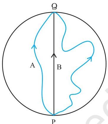 Fig. 3.19
3.9 Consider a cyclist who commences their journey from the central point $O$ of a circular park, which has a radius of $1\mathrm{km}$. They proceed to the park's periphery at point $P$, then navigate along the circular boundary, ultimately returning to the center via path $QO$, as illustrated in Fig. 3.20. Given that this entire circuit requires $10\mathrm{min}$, determine the cyclist's (a) overall displacement, (b) mean velocity, and (c) mean speed.
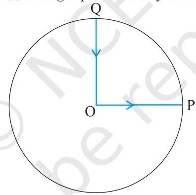 Fig. 3.20
3.10 A motorist navigates an open terrain along a route that consistently involves a $60^{\circ}$ leftward turn after each $500\mathrm{m}$ segment. Beginning from an arbitrary initial turn, identify the motorist's displacement at the third, sixth, and eighth turns. For each instance, contrast the magnitude of this displacement with the cumulative distance traversed by the motorist. 3.11 Upon reaching an unfamiliar town, a traveler desires to reach a hotel situated $10\mathrm{km}$ directly along a straight road from the station. However, an unscrupulous taxi driver transports the passenger via a circuitous route measuring $23\mathrm{km}$ in length, arriving at the hotel after $28\mathrm{min}$. Calculate (a) the taxi's mean speed and (b) the magnitude of its mean velocity. Do these two quantities possess identical values? 3.12 A prolonged hall features a ceiling at an elevation of $25\mathrm{m}$. Determine the greatest horizontal range achievable by a ball launched with an initial speed of $40\mathrm{ms}^{-1}$ such that it does not strike the hall's ceiling. 3.13 A cricketer is capable of propelling a ball to a maximum horizontal range of $100\mathrm{m}$. What is the maximum vertical height to which this same ball can be thrown by the cricketer?
3.14 An object, specifically a stone, is fastened to the extremity of an $80\mathrm{cm}$ string and is rotated uniformly in a horizontal circular path. If the stone completes $14$ full rotations within $25\mathrm{s}$, what are the magnitude and directional attributes of the stone's acceleration?
3.15 An aircraft performs a horizontal circular maneuver with a radius of $1.00\mathrm{km}$ while maintaining a constant speed of $900\mathrm{km/h}$. Evaluate its centripetal acceleration in relation to the acceleration caused by gravity.
3.16 Read each statement below carefully and state, with reasons, if it is true or false:
(a) For a particle undergoing circular motion, its resultant acceleration consistently points along the radius of the circle, directed towards its center. (b) The velocity vector associated with a particle at any given point is invariably oriented tangentially to the particle's trajectory at that specific location. (c) When considering a particle in uniform circular motion, the average acceleration vector computed over a single complete cycle results in a null vector.
3.17 The position of a particle is given by
$ \mathbf{r} = 3.0t \hat{\mathbf{i}} - 2.0t^2 \hat{\mathbf{j}} + 4.0 \hat{\mathbf{k}} \mathbf{m} $
where $t$ is expressed in seconds, and the numerical coefficients possess the appropriate units to ensure that $\mathbf{r}$ is represented in meters.
(a) Determine the velocity vector $\mathbf{v}$ and the acceleration vector $\mathbf{a}$ of the particle. (b) Calculate the magnitude and specify the direction of the particle's velocity at the instant $t = 2.0$ s.
3.18 A particle initiates its motion from the origin at $t = 0$ s, possessing an initial velocity of $10.0 , \text{km/s}$, and subsequently traverses the $x-y$ plane under the influence of a constant acceleration given by $(8.0 \hat{\mathbf{i}} + 2.0 \hat{\mathbf{j}}) , \text{m/s}^2$. (a) At what specific time will the particle's $x$-coordinate attain a value of $16 , \text{m}$? Furthermore, what will be the corresponding $y$-coordinate of the particle at that precise moment? (b) Ascertain the speed of the particle at this determined time.
3.19 Consider $\hat{\mathbf{i}}$ and $\hat{\mathbf{j}}$ as orthogonal unit vectors defining the $x-$ and $y-$axes, respectively. Determine both the magnitude and the orientation for the vector sums $\hat{\mathbf{i}} + \hat{\mathbf{j}}$ and $\hat{\mathbf{i}} - \hat{\mathbf{j}}$. Furthermore, calculate the scalar components of the vector $\mathbf{A} = 2\hat{\mathbf{i}} + 3\hat{\mathbf{j}}$ projected onto the directions specified by $\hat{\mathbf{i}} + \hat{\mathbf{j}}$ and $\hat{\mathbf{i}} - \hat{\mathbf{j}}$. [You may use graphical method]
3.20 Among the following expressions, identify which are valid for any general three-dimensional motion:
(a) $\mathbf{v}{\text{average}} = (1/2)(\mathbf{v}(t_1) + \mathbf{v}(t_2))$ (b) $\mathbf{v}{\text{average}} = [\mathbf{r}(t_2) - \mathbf{r}(t_1)] / (t_2 - t_1)$ (c) $\mathbf{v}(t) = \mathbf{v}(0) + \mathbf{a}t$ (d) $\mathbf{r}(t) = \mathbf{r}(0) + \mathbf{v}(0)t + (1/2)\mathbf{a}t^2$ (e) $\mathbf{a}_{\text{average}} = [\mathbf{v}(t_2) - \mathbf{v}(t_1)] / (t_2 - t_1)$
(Here, 'average' refers to the mean value of the specified quantity over the time duration from $t_1$ to $t_2$)
3.21 Examine each assertion provided below meticulously and indicate, supported by justifications and illustrative examples, whether it holds true or false:
A scalar quantity is characterized by the property that it:
(a) remains invariant throughout a given process (b) is incapable of assuming negative numerical values (c) inherently possesses no physical dimensions (d) maintains a uniform value across all spatial locations (e) presents an identical measure to observers utilizing distinct coordinate system orientations.
3.22 An airplane maintains a constant altitude of $3400,\mathrm{m}$ above the Earth's surface. From a fixed vantage point on the ground, the angular separation between two positions of the aircraft, recorded $10.0,\mathrm{s}$ apart, is observed to be $30^\circ$. Determine the velocity of the aircraft.