CHAPTER FOURTEEN
WAVES
14.1 Introduction
14.2 Transverse and longitudinal waves
14.3 Displacement relation in a progressive wave
14.4 The speed of a travelling wave
14.5 The principle of superposition of waves
14.6 Reflection of waves
14.7 Beats
Summary
Points to ponder
Exercises
14.1 INTRODUCTION
In the preceding Chapter, our focus was on the independent oscillatory motion of individual objects. We now consider the behavior within a system composed of numerous such entities. A material medium serves as an illustrative instance where constituent particles are interconnected by elastic forces, meaning the movement of one influences the others. Consider the effect of dropping a small pebble into a calm body of water; the surface experiences a disturbance. This perturbation does not localize but radiates outwards in a circular pattern. If pebbles are continuously introduced, one observes concentric circles rapidly expanding from the point of impact. This might suggest the water itself is flowing outwards from the disturbance's origin. However, if pieces of cork are placed on the affected surface, they are seen to oscillate vertically without drifting away from the disturbance's center. This observation demonstrates that the water mass does not physically move outwards with the expanding circles; instead, a propagating disturbance is generated. Similarly, when speech occurs, sound emanates outwards from the source without any bulk displacement of air from one region of the medium to another. The disturbances generated in air are considerably less apparent, discernible only by the human ear or through a microphone. These patterns, which advance without the actual physical relocation or bulk flow of matter, are termed waves. This Chapter is dedicated to the study of such phenomena.
Waves serve to transmit energy, and the configuration of the disturbance carries information that propagates across space. Fundamentally, all our communication relies on the transmission of signals via waves. Speech, for example, involves the creation of sound waves in the atmosphere, and hearing constitutes their detection. Frequently, communication processes incorporate various types of waves. For instance, sound waves might initially be converted into an electrical current signal, which could then generate an electromagnetic wave suitable for transmission through an optical fiber or via a
satellite link. The recovery of the original signal typically involves these stages in reverse sequence.
It is not universally true that waves necessitate a medium for their propagation. Light waves, as is well-known, possess the capacity to traverse a vacuum. The luminosity from stars, situated light-years distant, reaches Earth by travelling through interstellar space, which is essentially a vacuum.
The most commonly encountered wave types, such as oscillations on a taut string, surface disturbances on water, acoustic waves, and seismic tremors, are classified as mechanical waves. These waves are contingent upon a medium for their transmission and cannot propagate in a vacuum. Their mechanism involves the oscillation of the medium's constituent particles and is dependent on the elastic characteristics of that medium. Electromagnetic waves, which will be explored in Class XII, represent a distinct category. Electromagnetic waves do not inherently demand a medium for their travel; they are capable of propagating through a vacuum. Light, radio waves, and X-rays all fall under the umbrella of electromagnetic waves. In a vacuum, all electromagnetic waves exhibit the identical speed, denoted by $c$, the value of which is :
$ c = 299, 792, 458 \mathrm{ms}^{-1}. \tag{14.1} $
A third distinct category comprises what are termed Matter waves. These waves are intrinsically linked to the fundamental constituents of matter, such as electrons, protons, neutrons, atoms, and molecules. Their theoretical basis is rooted in the principles of quantum mechanics, a subject to be explored in advanced curricula. Despite their greater conceptual abstraction compared to mechanical or electromagnetic waves, they have already demonstrated practical utility in foundational modern technologies; notably, electron matter waves are harnessed in electron microscopy.
This chapter focuses on the investigation of mechanical waves, whose transmission necessitates the presence of a material medium.
While the aesthetic impact of waves on artistic and literary expression has been evident since antiquity, rigorous scientific inquiry into wave phenomena commenced in the seventeenth century. Pioneering figures in the study of wave physics include Christiaan Huygens (1629-1695), Robert Hooke, and Isaac Newton. The conceptualization of wave physics evolved from insights gained in the study of oscillatory systems, such as masses attached to springs and the simple pendulum. A fundamental relationship exists between waves propagating through elastic media and harmonic oscillations. (Examples of elastic media encompass stretched strings, coiled springs, and air).
We shall illustrate this connection through simple examples.
Let us consider an arrangement of interconnected springs, as depicted in Fig. 14.1. Upon abruptly displacing and releasing a spring at one extremity, the resulting perturbation propagates along the chain to the opposite end. What has
 Fig. 14.1 A collection of springs connected to each other. The end A is pulled suddenly generating a disturbance, which then propagates to the other end.
transpired? The initial spring is displaced from its equilibrium state. Given its connection to the first, the subsequent spring also undergoes stretching or compression, and this sequence continues along the array. The perturbation traverses the entire length, yet each individual spring merely performs minor oscillations around its own equilibrium point. To illustrate this phenomenon practically, consider a stationary train parked at a railway station. The various carriages (bogies) are interconnected via spring couplings. When an engine applies a thrust at one extremity, this impulse is imparted to the adjacent carriage and subsequently transmitted through the entire sequence of carriages, without the train as a whole undergoing significant bodily displacement.
Next, we examine the propagation mechanism of sound waves within an aerial medium. As a sound wave traverses air, it alternately compresses or rarefies localized volumes of the gas. This action results in a localized alteration in density, denoted as $\delta \rho$, which in turn precipitates a corresponding pressure variation, $\delta p$, within that volume. Given that pressure is defined as force per unit area, a restoring force arises, directly proportional to the magnitude of the disturbance, analogous to the behavior of a spring. Here, the analogue to a spring's extension or compression is the modification in density. When a specific region experiences compression, its constituent molecules become more closely packed, exhibiting a propensity to diffuse into adjacent areas, thereby elevating the density or inducing compression in those neighbouring regions. Conversely, the initial region then undergoes rarefaction. Should a region become comparatively rarefied, the ambient air flows inward, causing the rarefaction to shift to the contiguous region. Consequently, the alternating zones of compression and rarefaction propagate sequentially through the medium, facilitating the transmission of the disturbance through the air.
PHYSICS
The same principles can be applied to solid materials. In a crystalline solid, atoms or groups of atoms are arranged in a repeating lattice structure. Within this arrangement, each atom or atomic cluster maintains an equilibrium state, influenced by the forces exerted by its surrounding atoms. If one atom is displaced from its position while others remain fixed, it experiences restoring forces, precisely analogous to those in a spring. Therefore, atoms within a lattice can be conceptualized as endpoints connected by elastic elements, such as springs.
The subsequent sections of this chapter will explore various characteristic properties of waves.
14.2 TRANSVERSE AND LONGITUDINAL WAVES
As previously established, the motion of mechanical waves involves oscillations of the medium's constituent particles. If these constituent particles oscillate perpendicularly to the direction of wave propagation, the wave is classified as a transverse wave. Conversely, if their oscillations occur parallel to the direction of wave propagation, it is termed a longitudinal wave.
Fig.14.2 illustrates the propagation of a single pulse along a string, generated by a singular upward and downward jerk. If the string's length is considerably greater
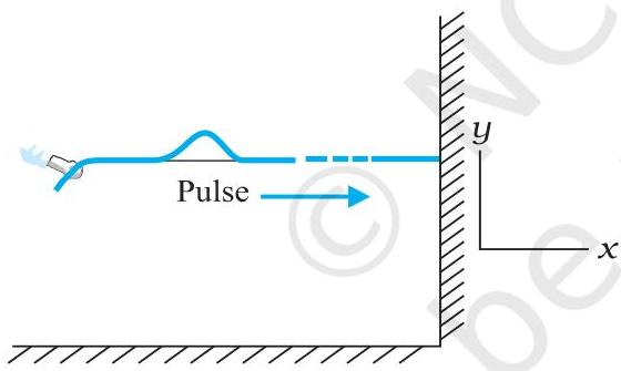 Fig. 14.2 When a pulse travels along the length of a stretched string (x-direction), the elements of the string oscillate up and down (y-direction)
than the size of the pulse, the pulse will attenuate before reaching the opposite end, and reflections from that end can be disregarded. Fig. 14.3 presents an analogous situation, but in this instance, the external agent applies a continuous, periodic sinusoidal upward and downward displacement to one end of the string. The resulting disturbance on the string is then a sinusoidal wave. In either case, the elements of the string oscillate about their equilibrium mean
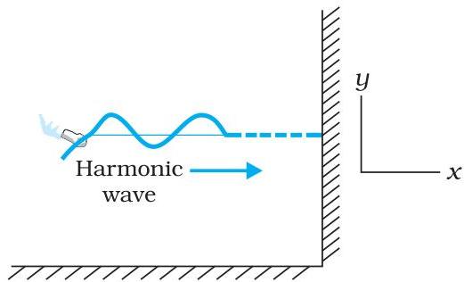 Fig. 14.3 A harmonic (sinusoidal) wave travelling along a stretched string is an example of a transverse wave. An element of the string in the region of the wave oscillates about its equilibrium position perpendicular to the direction of wave propagation.
position as the pulse or wave traverses their location. Given that these oscillations occur perpendicular to the direction of wave motion along the string, this phenomenon serves as an example of a transverse wave.
A wave can be examined from two distinct viewpoints. One can fix a particular instant in time and visualise the wave's spatial configuration. This provides a snapshot of the wave's overall shape in space at that given moment. Alternatively, one can fix a specific location—that is, focus attention on a particular element of the string—and observe its oscillatory motion over time.
Fig. 14.4 depicts the situation for longitudinal waves, using the most common illustration of sound wave propagation. An extended pipe filled with air features a piston at one end. A single, abrupt forward push and subsequent backward pull of the piston will generate a pulse composed of condensations (regions of higher density) and rarefactions (regions of lower density) within the medium (air). If the piston's push-pull action is continuous and periodic (sinusoidal), a
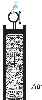 Fig. 14.4 Longitudinal (sound) waves produced within an air-filled pipe through the vertical displacement of a piston. An elemental volume of air undergoes oscillation in a direction parallel to the wave's propagation.
WAVES
Consequently, a sinusoidal wave will be produced that propagates through the air along the pipe's axis. This distinctly exemplifies longitudinal wave motion.
The previously discussed wave types, whether transverse or longitudinal, are categorised as travelling or progressive waves due to their propagation from one region of the medium to another. As previously established, the physical medium itself does not exhibit bulk displacement. For instance, a river's current represents the overall movement of water. Conversely, in a water wave, it is the perturbation that advances, not the entire body of water. Similarly, wind (the bulk flow of air) must not be mistaken for a sound wave, which involves the propagation of a disturbance (in pressure and density) through air without the overall transport of the air medium.
For transverse waves, the oscillatory movement of particles occurs perpendicularly to the wave's propagation direction. Consequently, with the wave's progression, each constituent element of the medium experiences a shearing strain. This implies that transverse waves are only capable of propagating in media that can withstand shearing stress, specifically solids, but not in fluids. Both fluids and solids are capable of sustaining compressive strain; hence, longitudinal waves are able to propagate through all elastic media. To illustrate, a medium like steel permits the propagation of both transverse and longitudinal waves, whereas air supports only longitudinal waves. Surface waves on water manifest in two primary categories: capillary waves and gravity waves. Capillary waves constitute ripples characterised by relatively short wavelengths—generally not exceeding a few centimetres—with surface tension acting as their restorative force. In contrast, gravity waves exhibit wavelengths typically spanning from several metres to several hundred metres. The gravitational force, which strives to maintain the water's surface at its lowest potential energy state, serves as the restoring mechanism for these waves. The particle oscillations within these waves are not restricted solely to the surface; rather, they penetrate to the very bottom, albeit with progressively decreasing amplitude. The kinematics of particles in water waves is intricate, encompassing both vertical (up and down) and horizontal (back and forth) displacements. Oceanic waves represent a composite of both longitudinal and transverse wave components.
It has been observed that, typically, transverse and longitudinal waves propagate at distinct velocities within the identical medium.
Example 14.1 The following are several instances of wave phenomena. For each case, identify whether the wave motion is transverse, longitudinal, or a hybrid of both: (a) Motion of a kink in a longitudinal spring produced by displacing one end of the spring sideways. (b) Waves produced in a cylinder containing a liquid by moving its piston back and forth. (c) Waves produced by a motorboat sailing in water. (d) Ultrasonic waves in air produced by a vibrating quartz crystal.
Answer
(a) Transverse and longitudinal (b) Longitudinal (c) Transverse and longitudinal (d) Longitudinal
14.3 DISPLACEMENT RELATION IN A PROGRESSIVE WAVE
To mathematically characterise a propagating wave, a function dependent on both spatial coordinate $x$ and temporal variable $t$ is essential. This function must, at any specific moment, define the wave's instantaneous profile. Concurrently, for any fixed spatial point, it must delineate the movement of the medium's element situated there. Should our aim be to represent a sinusoidal travelling wave (exemplified in Fig. 14.3), its descriptive function must inherently be sinusoidal. For analytical ease, we will assume a transverse wave, wherein if $x$ designates the position of the medium's constituent elements, their deviation from equilibrium can be represented by $y$. Consequently, a sinusoidal travelling wave is expressed as:
$ y(x,t) = a \sin(kx - \omega t + \phi) \tag{14.2} $
The presence of the term $\phi$ within the sine function's argument is mathematically equivalent to considering a linear superposition of sine and cosine functions:
$ y(x,t) = A \sin(kx - \omega t) + B \cos(kx - \omega t) \tag{14.3} $
From Equations (14.2) and (14.3),
$ a = \sqrt{A^2 + B^2} \quad \text{and} \quad \phi = \tan^{-1}\left(\frac{B}{A}\right) $
To grasp why Equation (14.2) indeed describes a sinusoidal travelling wave, consider a specific moment, for instance, $t = t_0$. In this scenario, the argument of the sine function in Equation (14.2) reduces to $
kx +$ a constant value. Consequently, the wave's form (at any given instant) as a spatial function $x$ is sinusoidal. Likewise, if we examine a fixed point, such as $x = x_0$, the sine function's argument in Equation (14.2) becomes a constant minus $\omega t$. Therefore, the displacement $y$ at a fixed location oscillates sinusoidally with time. This implies that the medium's elements at various positions undergo simple harmonic motion. Furthermore, for the phase $kx - \omega t + \phi$ to remain constant, an increase in $t$ necessitates a corresponding increase in $x$ in the positive direction. This demonstrates that Equation (14.2) characterises a sinusoidal (or harmonic) wave propagating along the positive $x$-axis. Conversely, a function expressed as:
$ y(x, t) = a \sin(kx + \omega t + \phi) \tag{14.4} $
signifies a wave propagating in the negative $x$-direction. Figure (14.5) outlines the definitions of the distinct physical parameters present in Equation (14.2), which we will now elucidate.
| $y(x,t)$ | : displacement as a function of position x and time t |
|---|---|
| $a$ | : amplitude of a wave |
| $\omega$ | : angular frequency of the wave |
| $k$ | : angular wave number |
| $kx - \omega t + \phi$ | : initial phase angle (at x = 0, t = 0) |
Fig. 14.5 The meaning of standard symbols in Eq. (14.2)
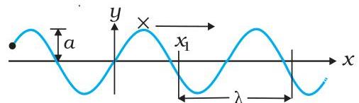
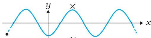
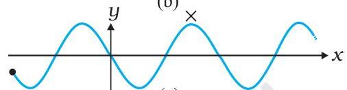
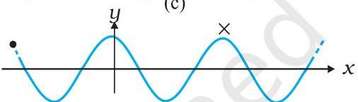
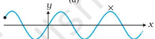
Figure 14.6 illustrates graphical representations of Equation (14.2) at various time instances, separated by uniform temporal intervals. Within a wave, the crest signifies the point of maximal positive displacement, while the trough denotes the point of maximal negative displacement. To observe wave propagation, one can focus on a crest and track its temporal advancement. This is indicated in the figure by a cross ( ) positioned on the crest. Analogously, the movement of a specific element of the medium at a stationary point, for instance, at the origin of the $x$-axis, can be monitored. This is depicted by a solid dot $(\bullet)$. The visualisations in Fig. 14.6 demonstrate that over time, the solid dot $(\bullet)$ at the origin undergoes periodic motion; that is, the particle at the origin oscillates around its equilibrium position as the wave advances. This phenomenon holds true for any other location as well. Furthermore, it is apparent that by the time the solid dot $(\bullet)$ completes one full oscillation, the crest has advanced by a specific distance.
 (a)
(a)
 (e)
Fig. 14.6 A harmonic wave progressing along the positive direction of $x$-axis at different times.
(e)
Fig. 14.6 A harmonic wave progressing along the positive direction of $x$-axis at different times.
Based on the graphical representations in Fig. 14.6, we will now delineate the distinct parameters comprising Eq. (14.2).
14.3.1 Amplitude and Phase
Within the framework of Eq. (14.2), the displacement $y(x,t)$ oscillates between the values of $a$ and $-a$, a direct consequence of the sine function's range from 1 to $-1$. It is conventional and mathematically sound to regard $a$ as a positive constant. In this context, $a$ signifies the maximal displacement experienced by the constituent particles of the medium from their equilibrium state. While the displacement $y$ itself can assume either positive or negative values, the quantity $a$ is inherently positive. This value $a$ is designated as the wave's amplitude.
The expression $(kx - \omega t + \phi)$, which acts as the argument for the sine function in Eq. (14.2), is termed the wave's phase. This phase, in conjunction with the amplitude $a$, uniquely specifies the wave's displacement at any given spatial coordinate and temporal instant. Specifically, $\phi$ represents the phase when both $x = 0$ and $t = 0$. Consequently, $\phi$ is referred to as the initial phase angle. It is feasible to set $\phi = 0$ through an appropriate selection of the origin on the $x$-axis and the initial time point. Therefore, no generality is lost by omitting $\phi$, which means considering Eq. (14.2) with $\phi = 0$.
14.3.2 Wavelength and Angular Wave Number
The wavelength of a wave, commonly denoted by $\lambda$, is defined as the minimal spatial separation between any two points that are in the same phase. For ease of understanding, these points can be conceptualised as consecutive crests or troughs. Therefore, the wavelength represents the distance spanning two adjacent crests or troughs within a wave pattern. By setting the phase constant $\phi = 0$ in Eq. (14.2), the displacement at a specific instant $t = 0$ can be expressed as:
$ y(x, 0) = a \sin kx \tag{14.5} $
Considering that the sine function exhibits periodicity, repeating its values after every $2\pi$ angular change, we can write:
$ \sin kx = \sin (kx + 2n\pi) = \sin k\left(x + \frac{2n\pi}{k}\right) $
This relationship implies that identical displacements occur at a position $x$ and at
$ x + \frac{2n\pi}{k} $
where $n = 1,2,3,\ldots$. The wavelength $\lambda$, which signifies the shortest distance between points exhibiting identical displacement at a given time, is determined by setting $n = 1$. Consequently, $\lambda$ is given by the formula:
$ \lambda = \frac{2\pi}{k} \quad \text{or} \quad k = \frac{2\pi}{\lambda} \tag{14.6} $
The parameter $k$ is referred to as the angular wave number or the propagation constant. Its SI unit is radian per metre, frequently written as
rad m$^{-1}$
14.3.3 Period, Angular Frequency and Frequency
Fig. 14.7 once more presents a sinusoidal representation. This depiction illustrates the displacement over time for a specific element of the medium (at a constant position), rather than portraying the instantaneous shape of the wave. To simplify, we can use Eq. (14.2) setting $\phi = 0$ and observe the behavior of the element at, for instance, $x = 0$. This yields:
$ \begin{array}{l} y(0, t) = a \sin (-\omega t) \ = -a \sin \omega t \end{array} $
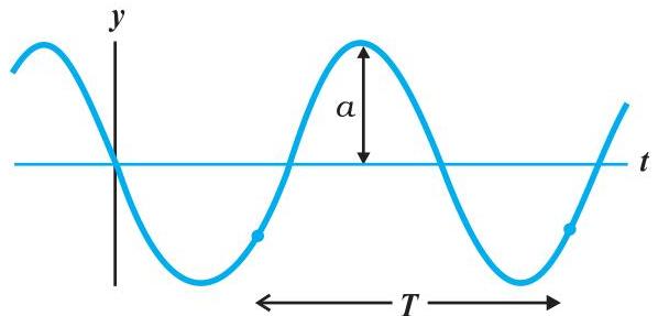 Fig. 14.7 A string element at a constant position oscillates with amplitude $a$ and period $T$ as the wave propagates.
The oscillation period of the wave is subsequently defined as the duration required for a medium element to execute a complete cycle of oscillation. This implies:
$ \begin{array}{l}
- a \sin \omega t = -a \sin \omega (t + T) \ = -a \sin (\omega t + \omega T) \end{array} $
Given that the sine function exhibits periodicity every $2\pi$ radians,
$ \omega T = 2\pi \quad \text{or} \quad \omega = \frac{2\pi}{T} \tag{14.7} $
The quantity $\omega$ is designated as the angular frequency of the wave, and its standard SI unit is rad s$^{-1}$. The frequency, denoted by $\nu$, represents the number of complete oscillations occurring per unit time (specifically, per second). Consequently,
$ \nu = \frac{1}{T} = \frac{\omega}{2\pi} \tag{14.8} $
The frequency $\nu$ is conventionally quantified in hertz.
Throughout the preceding discussion, the focus has consistently been on waves propagating along a string, characteristic of transverse waves. Conversely, in the context of a longitudinal wave, the displacement undergone by an element of the medium occurs in a direction parallel to the wave's propagation. For a longitudinal wave, the displacement function, analogous to Eq. (14.2), is expressed as:
$ s(x, t) = a \sin (kx - \omega t + \phi) \tag{14.9} $
Here, $s(x, t)$ denotes the displacement of a medium element situated at position $x$ at time $t$, specifically along the direction of wave propagation. Within Eq. (14.9), $a$ signifies the displacement amplitude; all other parameters maintain the identical interpretations as those established for a transverse wave, with the sole distinction being the substitution of the displacement function $y(x, t)$ with $s(x, t)$.
Example 14.2: Consider a wave propagating along a string, characterised by the following expression:
$ y (x, t) = 0.005 \sin (80.0 , x - 3.0 , t), $
where the numerical coefficients are provided in SI units (0.005 m, 80.0 rad m$^{-1}$, and 3.0 rad s$^{-1}$). Determine (a) the amplitude, (b) the wavelength, and (c) the period and frequency of this wave. Furthermore, compute the displacement $y$ of the wave at a spatial coordinate $x = 30.0$ cm and a temporal instant $t = 20$ s.
Answer: Through a direct comparison of the given displacement equation with the general form presented in Eq. (14.2),
$ y (x, t) = a \sin (k x - \omega t), $
it is observed that:
(a) the wave's amplitude is $0.005,\mathrm{m}$, equivalent to $5,\mathrm{mm}$. (b) the angular wave number $k$ and the angular frequency $\omega$ are found to be:
$ k = 80.0 , \mathrm{m}^{-1} \text{ and } \omega = 3.0 , \mathrm{s}^{-1} $
Subsequently, we establish the relationship between the wavelength $\lambda$ and $k$ utilising Eq. (14.6):
$ \begin{array}{l} \lambda = 2 \pi / k \ = \frac{2 \pi}{80.0 , \mathrm{m}^{-1}} \ = 7.85 , \mathrm{cm} \end{array} $
(c) Now, we relate $T$ to $\omega$ by the relation
$ \begin{array}{l} T = 2 \pi / \omega \ = \frac{2 \pi}{3.0 , \mathrm{s}^{-1}} \ = 2.09 , \mathrm{s} \end{array} $
and frequency, $\nu = 1 / T = 0.48,\mathrm{Hz}$
The displacement $y$ at $x = 30.0$ cm and time $t = 20$ s is given by
$ \begin{array}{l} y = (0.005 , \mathrm{m}) \sin (80.0 \times 0.3 - 3.0 \times 20) \ = (0.005 , \mathrm{m}) \sin (-36 + 12\pi) \ = (0.005 , \mathrm{m}) \sin (1.699) \ = (0.005 , \mathrm{m}) \sin (97^{\circ}) \simeq 5 , \mathrm{mm} \end{array} $
14.4 THE SPEED OF A TRAVELLING WAVE
To ascertain the propagation velocity of a travelling wave, one can concentrate on any specific locus within the wave (defined by a constant phase value) and monitor its temporal displacement. Observing the crest's movement often proves advantageous. Figure 14.8 depicts the wave's configuration at two distinct moments, separated by a brief interval $\Delta t$. The complete wave morphology is observed to translate rightward (along the positive $x$-axis) by a distance $\Delta x$. Specifically, the crest, indicated by a dot $(\bullet)$, traverses a
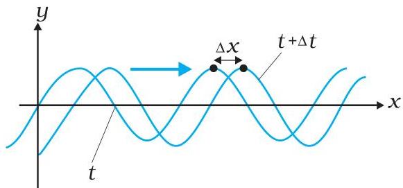 Fig. 14.8 Progression of a harmonic wave from time $t$ to $t + \Delta t$. where $\Delta t$ is a small interval. The wave pattern as a whole shifts to the right. The crest of the wave (or a point with any fixed phase) moves right by the distance $\Delta x$ in time $\Delta t$.
displacement $\Delta x$ over the time interval $\Delta t$. Consequently, the wave's velocity is defined as $\Delta x / \Delta t$. One could equally place the marker $(\bullet)$ on a point exhibiting any other constant phase; this point would also advance at the identical speed $\nu$, as any deviation would result in a distortion of the wave pattern. The kinematic behavior of a point possessing a constant phase on the wave is mathematically represented by
$ k x - \omega t = \text{constant} \tag{14.10} $
Hence, for the phase to persist as constant, the spatial coordinate $x$ of the fixed-phase point must adjust commensurately with changes in time $t$. This implies:
$ k x - \omega t = k (x + \Delta x) - \omega (t + \Delta t) $
or $k\Delta x - \omega \Delta t = 0$
As $\Delta x$ and $\Delta t$ approach infinitesimal values, this relationship yields
$ \frac{dx}{dt} = \frac{\omega}{k} = v \tag{14.11} $
By establishing the connections between $\omega$ and $T$, and $k$ and $\lambda$, the following expression is derived:
$ v = \frac{2 \pi \nu}{2 \pi / \lambda} = \lambda \nu = \frac{\lambda}{T} \tag{14.12} $
Equation (14.12), which applies universally to all progressive waves, illustrates that within the duration of a single complete oscillation by any element of the propagating medium, the entire wave configuration advances a distance equivalent to its wavelength. It is imperative to recognise that the velocity of a mechanical wave is fundamentally governed by the medium's inherent inertial characteristics (such as linear mass density for string systems, or mass density more broadly) and its elastic moduli (e.g., Young's modulus for one-dimensional continua, or shear and bulk moduli for more general cases). The intrinsic properties of the medium dictate the wave's
speed; subsequently, Equation (14.12) establishes the relationship between wavelength and frequency for that specific velocity. As previously indicated, a given medium is capable of sustaining both transverse and longitudinal wave modes, each of which will typically exhibit distinct propagation speeds within the same material. Subsequent sections of this chapter will present explicit formulations for the velocities of mechanical waves in various specific media.
14.4.1 Speed of a Transverse Wave on Stretched String
The propagation velocity of a mechanical wave within a medium is governed by two principal characteristics: the magnitude of the restoring force generated upon disturbance and the medium's inherent inertial attributes (specifically, its mass density). It is generally anticipated that this velocity will exhibit a direct correlation with the restoring force and an inverse relationship with the inertial properties. In the context of waves propagating along a string, the requisite restoring force originates from the tension, denoted as $T$, present in the string. The relevant inertial characteristic for this scenario is the linear mass density, $\mu$, which represents the string's mass $m$ distributed over its length $L$. While a precise mathematical expression for the wave speed on a string can be formulated through the application of Newton's Laws of Motion, such a derivation falls outside the purview of this text. Consequently, our approach will involve dimensional analysis. It is important to recall that dimensional analysis inherently cannot yield a complete, exact formula, as any dimensionless constant factor invariably remains unresolved by this method.
The dimensional representation for the linear mass density $\mu$ is $[ML^{-1}]$, while that for tension $T$ aligns with the dimensions of force, specifically $[MLT^{-2}]$. Our objective is to combine these dimensions to arrive at the dimension for speed, $\nu$, which is $[LT^{-1}]$. A straightforward examination reveals that the ratio $T / \mu$ possesses the appropriate combined dimensions, as demonstrated below:
$ \left[ \frac {M L T ^ {- 2}}{M L} \right] = \left[ L ^ {2} T ^ {- 2} \right] $
Therefore, assuming that $T$ and $\mu$ are the sole pertinent physical quantities, the wave speed can be expressed as:
$ \nu = C \sqrt {\frac {T}{\mu}} \tag {14.13} $
Here, $C$ denotes the dimensionless constant that remains indeterminate through dimensional analysis. It is subsequently revealed in the precise formulation that this constant $C$ equals 1. Consequently, the speed of transverse waves on a stretched string is accurately given by:
$ \nu = \sqrt {\frac {T}{\mu}} \tag {14.14} $
It is crucial to observe that the wave speed, $\nu$, is solely contingent upon the intrinsic characteristics of the medium—namely, the tension $T$ and the linear mass density $\mu$. (It is important to clarify that $T$ itself is a property of the stretched string, resulting from an external force application.) This speed exhibits no dependence on the wavelength or the frequency of the wave itself. Advanced studies will introduce scenarios involving waves whose propagation speed is indeed frequency-dependent. Considering the two fundamental wave parameters, wavelength ($\lambda$) and frequency (here denoted as $\nu$), the frequency of the generated wave is determined exclusively by its source of disturbance. Given the wave's speed in the medium (represented as $v$) and its frequency ($\nu$), the wavelength is subsequently established by the relationship:
$ \lambda = \frac {v}{\nu} \tag {14.15} $
Example 14.3 A steel wire $0.72\mathrm{m}$ long has a mass of $5.0\times 10^{-3}\mathrm{kg}$. If the wire is under a tension of $60\mathrm{N}$, what is the speed of transverse waves on the wire?
Answer The linear mass density of the wire, calculated as mass per unit length, is determined as follows:
$ \begin{array}{l} \mu = \frac {5 . 0 \times 1 0 ^ {- 3} \mathrm {k g}}{0 . 7 2 \mathrm {m}} \ = 6. 9 \times 1 0 ^ {- 3} \mathrm {k g} \mathrm {m} ^ {- 1} \ \end{array} $
The applied tension, $T$, is $60\mathrm{N}$.
The propagation speed of the wave along the wire is then calculated using the established formula:
$ v = \sqrt {\frac {T}{\mu}} = \sqrt {\frac {6 0 \mathrm {N}}{6 . 9 \times 1 0 ^ {- 3} \mathrm {k g} \mathrm {m} ^ {- 1}}} = 9 3 \mathrm {m} \mathrm {s} ^ {- 1} $
14.4.2 Speed of a Longitudinal Wave (Speed of Sound)
Within a longitudinal wave, the constituent particles of the transmitting medium undergo oscillatory motion, displacing back and forth along the same axis as the wave's propagation. As previously established, sound waves propagate through the formation of localised regions of increased (compressions) and decreased (rarefactions) density within small volumetric elements of the air. The elastic characteristic governing the stress response to a compressional deformation is the medium's bulk modulus, as introduced in Chapter 8 and defined as follows:
$ B = - \frac {\Delta P}{\Delta V / V} \tag {14.16} $
In this expression, the pressure variation, $\Delta P$, elicits a corresponding fractional change in volume, $\frac{\Delta V}{V}$. The bulk modulus, $B$, shares the same dimensional characteristics as pressure and is quantified in SI units using pascals (Pa). For wave propagation, the pertinent inertial attribute is the mass density, $\rho$, possessing dimensions of $[ML^{-3}]$. A straightforward dimensional analysis indicates that the ratio $B / \rho$ yields dimensions suitable for a wave speed:
$
\frac {\left[ M L ^ {- 2} T ^ {- 2} \right]}{\left[ M L ^ {- 3} \right]} = \left[ L ^ {2} T ^ {- 2} \right] \tag {14.17} $
Consequently, assuming $B$ and $\rho$ constitute the sole influential physical parameters, the wave speed can be expressed as:
$ \nu = C \sqrt {\frac {B}{\rho}} \tag {14.18} $
Here, $C$ represents the dimensionless constant whose value remains indeterminate through dimensional analysis alone. However, a rigorous derivation reveals that $C = 1$. Hence, the universal equation for the velocity of longitudinal waves in a given medium becomes:
$ \nu = \sqrt {\frac {B}{\rho}} \tag {14.19} $
Considering a linear medium, such as a solid rod, where transverse expansion is negligible, the material can be treated as being subjected exclusively to longitudinal strain. In this specific scenario, the appropriate elastic modulus is Young's modulus, which possesses identical dimensions to the bulk modulus. Applying dimensional analysis similarly to the preceding case results in an analogous relationship to Eq. (14.18), incorporating an undetermined constant $C$, subsequently confirmed as unity by precise derivation. Accordingly, the velocity of longitudinal waves through a solid bar is determined by:
$ \nu = \sqrt {\frac {Y}{\rho}} \tag {14.20} $
where $Y$ denotes the Young's modulus pertinent to the bar's constituent material. Table 14.1 presents typical speeds of sound in various media.
Table 14.1 Speed of Sound in some Media
| Medium | Speed (m s^{-1}) |
|---|---|
| Gases | |
| Air (0 °C) | 331 |
| Air (20 °C) | 343 |
| Helium | 965 |
| Hydrogen | 1284 |
| Liquids | |
| Water (0 °C) | 1402 |
| Water (20 °C) | 1482 |
| Seawater | 1522 |
| Solids | |
| Aluminium | 6420 |
| Copper | 3560 |
| Steel | 5941 |
| Granite | 6000 |
| Vulcanised | |
| Rubber | 54 |
Typically, the propagation velocity of sound is greater in liquids and solids compared to gases. (It is important to note that for solid materials, this speed specifically pertains to longitudinal waves within the solid). This phenomenon arises from the considerably higher resistance of liquids and solids to compression relative to gases, resulting in substantially elevated bulk modulus values. Referring to Eq. (14.19), while solids and liquids exhibit greater mass densities $(\rho)$ than gases, the proportional increase in their respective moduli $(B)$ is significantly more pronounced. This differential increase accounts for the accelerated travel of sound waves through solid and liquid media.
The velocity of sound in a gas can be approximated using the ideal gas model. For an ideal gas, the relationship between its pressure $P$, volume $V$, and temperature $T$ is defined by (refer to Chapter 10):
$ P V = N k _ {B} T \tag {14.21} $
Here, $N$ represents the total count of molecules within volume $V$, $k_{B}$ denotes the Boltzmann constant, and $T$ signifies the absolute temperature of the gas (in Kelvin). Consequently, for a process occurring under isothermal conditions, it can be deduced from Eq. (14.21) that:
$ V \Delta P + P \Delta V = 0 $
or, rearranged, $-\frac{\Delta P}{\Delta V / V} = P$.
Therefore, by substituting this into Eq. (14.16), we obtain:
$ B = P $
From this, and referring to Eq. (14.19), the speed of a longitudinal wave propagating through an ideal gas is expressed as:
$ \nu = \sqrt {\frac {P}{\rho}} \tag {14.22} $
This relationship, initially proposed by Newton, is widely recognised as Newton's formula.
Example 14.4 Estimate the speed of sound in air at standard temperature and pressure. The mass of 1 mole of air is $29.0 \times 10^{-3} \mathrm{~kg}$ .
Answer It is established that one mole of any gas occupies 22.4 litres at STP. Thus, the density of air at STP can be calculated as:
$\rho_{o} =$ (mass of one mole of air) / (volume of one mole of air at STP)
$ \begin{array}{l} = \frac {2 9 . 0 \times 1 0 ^ {- 3} \mathrm {k g}}{2 2 . 4 \times 1 0 ^ {- 3} \mathrm {m} ^ {3}} \ = 1. 2 9 \mathrm {k g} \mathrm {m} ^ {- 3} \ \end{array}
$
Applying Newton's formula for the speed of sound within a medium, the sound velocity in air at STP is computed as:
$ v = \left[ \frac {1.01 \times 10^{5} \mathrm{N} \mathrm{m}^{-2}}{1.29 \mathrm{kg} \mathrm{m}^{-3}} \right]^{1/2} = 280 \mathrm{m} \mathrm{s}^{-1} \tag{14.23} $
The value presented in Eq. (14.23) is approximately $15%$ lower than the experimentally determined value of $331\mathrm{ms}^{-1}$, as cited in Table 14.1. This discrepancy prompts a re-evaluation of the underlying assumptions. Newton's initial premise, that pressure variations accompanying sound propagation in a medium are isothermal, proves to be inaccurate upon closer examination. Laplace correctly identified that the rapid nature of pressure fluctuations during sound wave propagation leaves insufficient time for heat exchange to maintain a constant temperature. Consequently, these variations are adiabatic rather than isothermal. For adiabatic processes, an ideal gas adheres to the following relation (as detailed in Section 11.8):
$ PV^{\gamma} = \text{constant} $
which implies $\Delta (PV^{\gamma}) = 0$.
This further expands to $P\gamma V^{\gamma -1}\Delta V + V^{\gamma}\Delta P = 0$.
Here, $\gamma$ represents the ratio of the two specific heats, $C_{\mathrm{p}} / C_{\mathrm{v}}$.
Therefore, for an ideal gas, the adiabatic bulk modulus is defined as:
$ \begin{array}{l} B_{ad} = - \frac{\Delta P}{\Delta V / V} \ = \gamma P \end{array} $
Thus, the speed of sound, derived from Eq. (14.19), is expressed as:
$ v = \sqrt{\frac{\gamma P}{\rho}} \tag{14.24} $
This refinement of Newton's formula is known as the Laplace correction. For air, the value of $\gamma$ is approximately $7/5$. By employing Eq. (14.24) to calculate the speed of sound in air at STP, we arrive at a value of $331.3\mathrm{ms}^{-1}$, which closely matches the experimentally observed speed.
14.5 THE PRINCIPLE OF SUPERPOSITION OF WAVES
Consider the interaction when two distinct wave pulses propagate towards each other from opposing directions (Fig. 14.9). Observations indicate that these wave pulses maintain their individual characteristics subsequent to their intersection. Nevertheless, during their period of spatial overlap, the composite wave configuration deviates from that of either individual pulse.
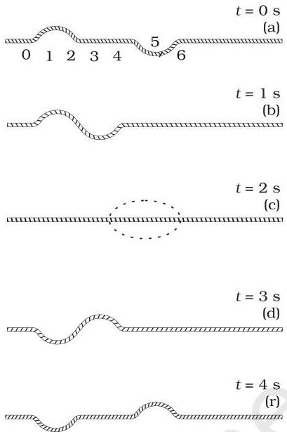 Fig. 14.9 Two pulses having equal and opposite displacements moving in opposite directions. The overlapping pulses add up to zero displacement in curve (c).
Figure 14.9 illustrates a scenario involving two pulses possessing identical yet oppositely directed displacements as they approach one another. Upon their convergence and overlap, the aggregate displacement observed is the algebraic sum of the displacements contributed by each constituent pulse. This fundamental concept is termed the principle of superposition of waves. In accordance with this principle, each individual pulse traverses the medium as if the other pulses were absent. Consequently, the medium's constituent elements experience displacements attributable to both pulses, and since these displacements can be either positive or negative, their cumulative effect manifests as an algebraic sum. Figure 14.9 presents graphical representations of the wave profile at various temporal instances, highlighting the notable phenomenon depicted in graph (c), where the displacements from the two pulses precisely nullify each other, resulting in a state of zero displacement across the entire region.
To express the principle of superposition in mathematical terms, let us denote $y_{1}(x,t)$ and $y_{2}(x,t)$ as the displacements produced by two distinct wave perturbations within a given medium. Should these waves concurrently enter and consequently overlap within a specific spatial domain, the resultant displacement, $y(x,t)$, is precisely articulated as:
$ y (x, t) = y _ {1} (x, t) + y _ {2} (x, t) \tag{14.25} $
Extending this concept, when multiple waves traverse the medium, the composite waveform is derived by summing the individual wave functions. Specifically, if the wave functions corresponding to the propagating waves are represented as:
$
y _ {1} = f _ {1} (x - v t), $
$ y _ {2} = f _ {2} (x - v t), $
$ \dots $
$ y _ {n} = f _ {n} (x - v t) $
then the wave function that characterises the overall disturbance within the medium becomes:
$ \begin{array}{l} y = f _ {1} (x - v t) + f _ {2} (x - v t) + \dots + f _ {n} (x - v t) \ = \sum_ {i = 1} ^ {n} f _ {i} (x - v t) \tag {14.26} \ \end{array} $
The principle of superposition is basic to the phenomenon of interference.
To simplify, let us examine two harmonic travelling waves propagating along a stretched string. We stipulate that both waves possess identical $\omega$ (angular frequency) and $k$ (wave number), which consequently implies they share the same wavelength $\lambda$. Their propagation velocities will, therefore, be equivalent. Furthermore, we shall assume their amplitudes are equal and that both are advancing along the positive $x$-axis. The sole distinction between these waves lies in their initial phase. As per Eq. (14.2), these two waves are characterised by the following functional forms:
$ y _ {1} (x, t) = a \sin (k x - \omega t) \tag {14.27} $
$ \text {and} y _ {2} (x, t) = a \sin (k x - \omega t + \phi) \tag {14.28} $
The net displacement is then, by the principle of superposition, given by
$ \begin{aligned} y(x,t) &= a \sin(kx - \omega t) + a \sin(kx - \omega t + \phi) \quad (14.29) \ &= 2a \cos\left(\frac{\phi}{2}\right)\sin\left(kx - \omega t + \frac{\phi}{2}\right) \quad (14.30) \end{aligned} $
By employing the well-known trigonometric identity for the sum of sines ($\sin A + \sin B$), we can transform the expression above to yield:
$ y (x, t) = 2 a \cos \frac {\phi}{2} \sin (k x - \omega t + \frac {\phi}{2}) \tag {14.31} $
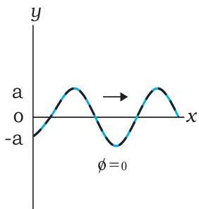
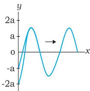
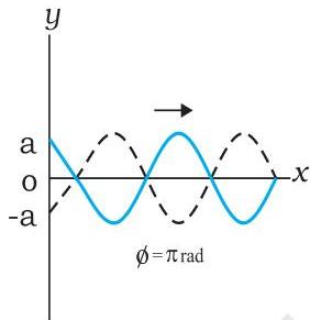
Equation (14.31) represents a harmonic travelling wave, propagating along the positive $x$-axis, retaining the original frequency and wavelength. However, its initial phase angle is now $\frac{\phi}{2}$. Crucially, the amplitude of this resultant wave is contingent upon the phase difference, denoted as $\phi$, between the two constituent waves:
 (a)
(a)
 (b)
(b)
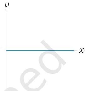 Fig. 14.10 The resultant of two harmonic waves of equal amplitude and wavelength according to the principle of superposition. The amplitude of the resultant wave depends on the phase difference $\phi$ , which is zero for (a) and $\pi$ for (b)
$ A (\phi) = 2 a \cos \frac {1}{2} \phi \tag {14.32} $
Consider the scenario where $\phi = 0$, signifying that the waves are perfectly in phase:
$ y (x, t) = 2 a \sin (k x - \omega t) \tag {14.33} $
In this instance, the resultant wave exhibits an amplitude of $2a$, which constitutes the maximum possible value for $A$. Conversely, when $\phi = \pi$, the waves are entirely out of phase, leading to a resultant wave with zero displacement across all spatial positions and at all temporal instances:
$ y (x, t) = 0 \tag {14.34} $
Equation (14.33) illustrates what is termed constructive interference between the two waves, where their amplitudes combine additively to form the resultant wave. Conversely, Equation (14.34) exemplifies destructive interference, a condition where the amplitudes effectively cancel each other out in the composite wave. Figure 14.10 visually depicts these two distinct interference phenomena, which arise from the principle of superposition.
14.6 REFLECTION OF WAVES
Up to this point, our discussion has centred on waves propagating within an unbounded medium. The question arises: what occurs when a pulse or a wave encounters a boundary? Should the boundary be rigid, the pulse or wave
undergoes reflection. A common instance of reflection from a rigid boundary is the phenomenon of an echo. When the boundary is not entirely rigid, or if it represents an interface between two distinct elastic media, the situation becomes more intricate. In such cases, a portion of the incident wave is reflected, while another part is transmitted into the second medium. If a wave impinges obliquely upon the interface separating two different media, the transmitted wave is designated as the refracted wave. The incident and refracted waves adhere to Snell's law of refraction, and the incident and reflected waves conform to the conventional laws of reflection.
Figure 14.11 illustrates a pulse propagating along a taut string and subsequently reflecting off a boundary. Assuming no energy is absorbed by the boundary, the reflected wave retains the identical shape of the incident pulse, but it experiences a phase alteration of $\pi$ radians or $180^{\circ}$ upon reflection. This occurs because the boundary is rigid, necessitating that the disturbance maintain zero displacement at that boundary at all times. According to the principle of superposition, this condition can only be satisfied if the reflected and incident waves differ in phase by $\pi$, thereby ensuring a resultant displacement of zero. This rationale is founded on the boundary condition applicable to a rigid wall. The same conclusion can also be reached through a dynamic analysis. As the pulse reaches the wall, it exerts a force upon it. By virtue of Newton's Third Law, the wall imparts an equal and opposite force back onto the string, thereby generating a reflected pulse that exhibits a phase difference of $\pi$.
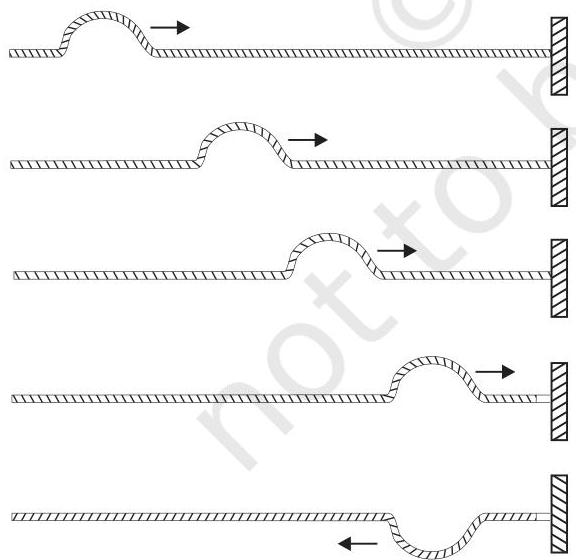 Fig. 14.11 Reflection of a pulse meeting a rigid boundary.
Conversely, if the boundary point is not rigid but instead entirely free to move (as exemplified by a string attached to a freely sliding ring on a rod), the reflected pulse possesses the same phase and amplitude as the incident pulse, assuming no energy dissipation. In this scenario, the total maximum displacement at the boundary becomes twice the amplitude of each individual pulse. An example of a non-rigid boundary is the open end of an organ pipe.
In summary, a propagating wave or pulse undergoes a phase shift of $\pi$ radians when reflected from a rigid boundary, whereas no phase change occurs upon reflection from an open boundary. Expressing this mathematically, let the incident travelling wave be represented by
$ y _ {2} (x, t) = a \sin (k x - \omega t) $
For a rigid boundary, the reflected wave is described by
$ \begin{array}{l} y _ {1} (x, t) = a \sin (k x - \omega t + \pi). \ = - a \sin (k x - \omega t) \tag {14.35} \ \end{array} $
For an open boundary, the reflected wave is given by
$ \begin{array}{l} y _ {1} (x, t) = a \sin (k x - \omega t + 0). \ = a \sin (k x - \omega t) \tag {14.36} \ \end{array} $
Evidently, at the rigid boundary, the total displacement $y = y_{2} + y_{r}$ remains zero at all instants.
14.6.1 Standing Waves and Normal Modes
Our previous discussion focused on wave reflection at a single interface. However, common scenarios exist—such as a string secured at both termini or an air column within a pipe with both ends sealed—where reflection occurs at two or more boundaries. For instance, in a string, a wave propagating in one direction will undergo reflection at one end; this reflected wave then travels to the opposing end, where it is reflected again. This iterative reflection process continues until a stable wave configuration, known as a standing wave or stationary wave, is established on the string. To illustrate this phenomenon mathematically, let us consider a wave propagating in the positive $x$-direction and a corresponding reflected wave, possessing identical amplitude and wavelength, moving in the negative $x$-direction. Based on Eqs. (14.2) and (14.4), assuming $\phi = 0$, we derive the following expressions:
$ \begin{array}{l} y _ {1} (x, t) = a \sin (k x - \omega t) \ y _ {2} (x, t) = a \sin (k x + \omega t) \ \end{array} $
In accordance with the principle of superposition, the resultant wave on the string is:
$ y (x, t) = y _ {1} (x, t) + y _ {2} (x, t) $
$
= a \left[ \sin (k x - \omega t) + \sin (k x + \omega t) \right] $
By employing the well-known trigonometric identity:
$\operatorname{Sin}(\mathrm{A} + \mathrm{B}) + \operatorname{Sin}(\mathrm{A} - \mathrm{B}) = 2\sin \mathrm{A}\cos \mathrm{B}$, we obtain:
$ y (x, t) = 2 a \sin k x \cos \omega t \tag {14.37} $
A crucial distinction exists between the wave pattern elucidated by Eq. (14.37) and those represented by Eq. (14.2) or Eq. (14.4). In Eq. (14.37), the spatial term $kx$ and the temporal term $\omega t$ are mathematically decoupled, rather than appearing as the combined argument $kx - \omega t$. Consequently, the amplitude of this resultant wave is expressed as $2a \sin kx$. This implies that within this wave configuration, the amplitude varies spatially, yet every constituent element of the string oscillates with an identical angular frequency $\omega$ or period. Significantly, there is an absence of phase difference among the oscillations of distinct wave elements. The entire string thus vibrates synchronously, albeit with amplitudes that differ depending on the specific location. This wave pattern exhibits no net propagation in either the positive or negative direction, which is why these phenomena are termed standing or stationary waves. While the amplitude remains constant at any particular position, it varies across different locations, as previously noted. Positions where the amplitude is zero (indicating no displacement) are designated as nodes, whereas points exhibiting maximum amplitude are referred to as antinodes. Figure 14.12 illustrates a characteristic stationary wave pattern arising from the superposition of two counter-propagating travelling waves.
A paramount characteristic of stationary waves is the imposition of constraints by boundary conditions on the permissible wavelengths or oscillation frequencies of the system. Unlike a harmonic travelling wave, which can exist at any frequency, the system is restricted to vibrating at a discrete set of intrinsic frequencies, termed natural frequencies or normal modes of oscillation. We shall now proceed to derive these normal modes for a taut string that is rigidly fixed at both extremities.
Initially, consulting Eq. (14.37), the locations of nodes (points of zero amplitude) are defined by the condition $\sin kx = 0$.
which implies
$ k x = n \pi ; \quad n = 0, 1, 2, 3, \dots $
By substituting $k = 2\pi /\lambda$, the resulting spatial positions are found to be:
$ x = \frac {n \lambda}{2}; n = 0, 1, 2, 3, \dots \tag {14.38} $
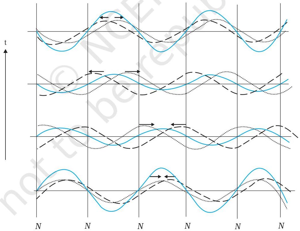 Fig. 14.12 Stationary waves arising from superposition of two harmonic waves travelling in opposite directions. Note that the positions of zero displacement (nodes) remain fixed at all times.
It is evident that the separation between consecutive nodes is $\frac{\lambda}{2}$. Similarly, the locations of antinodes, defined as points of maximum amplitude, are determined by the peak value of $\sin kx$:
$\left|\sin kx\right| = 1$
which implies
$ k x = (n + \frac {1}{2}) \pi ; n = 0, 1, 2, 3, \dots $
By substituting $k = 2\pi /\lambda$, we arrive at the following expression for the spatial coordinates:
$ x = (n + \frac {1}{2}) \frac {\lambda}{2}; n = 0, 1, 2, 3, \dots \tag {14.39} $
Furthermore, the spacing between any two adjacent antinodes also measures $\frac{\lambda}{2}$. Equation (14.38) is applicable to the scenario of a stretched string of length $L$ that is secured at both extremities. Assuming one end is located at $x = 0$, the imposed boundary conditions stipulate that both $x = 0$ and $x = L$ must correspond to nodal points. The condition at $x = 0$ is inherently met. However, the nodal requirement at $x = L$ mandates that the string's length $L$ must be related to the wavelength $\lambda$ through the expression:
$ L = n \frac {\lambda}{2}; \quad n = 1, 2, 3, \dots \tag {14.40} $
Consequently, the permissible wavelengths for stationary waves are restricted by the relationship:
$ \lambda = \frac {2 L}{n}; n = 1, 2, 3, \dots \tag{14.41} $
with their respective frequencies given by:
$ \nu = \frac {n v}{2 L}, \text {f o r} n = 1, 2, 3, \dots \tag{14.42} $
We have thereby derived the intrinsic frequencies, which represent the normal modes of oscillation characteristic of the system. The minimum achievable natural frequency for a system is designated as its fundamental mode or the first harmonic. In the context of a stretched string anchored at both ends, this is expressed as:
it is given by $\nu = \frac{v}{2L}$ , corresponding
to $n = 1$ of Eq. (14.42). In this formulation, $\nu$ denotes the wave propagation speed, which is intrinsically governed by the properties of the transmitting medium. The frequency associated with $n = 2$ is termed the second harmonic; similarly, $n = 3$ corresponds to the third harmonic, and this pattern continues. The various harmonics can be systematically denoted by the symbol $\nu_{ij} (n = 1, 2, \ldots)$.
Figure 14.13 illustrates the initial six harmonics generated by a stretched string with fixed endpoints. It is not mandatory for a string to oscillate exclusively in a single one of these modes. Typically, the vibrational behavior of a string manifests as a superposition of various modes; certain modes may be activated with greater intensity, while others are less pronounced. Musical instruments such as the sitar or violin operate on this fundamental principle. The specific location where the string is plucked or bowed dictates which particular modes achieve greater prominence relative to others.
We shall now proceed to examine the normal modes of oscillation within an air column that has one end closed.
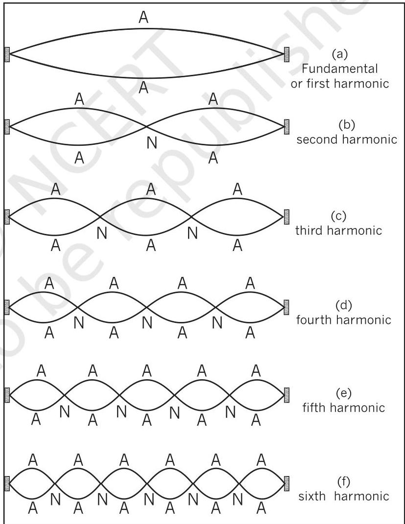 Fig. 14.13 The first six harmonics of vibrations of a stretched string fixed at both ends.
PHYSICS
A system characterised by one closed and one open end is exemplified by a glass tube containing some water. The interface where the tube meets the water acts as a node, whereas the unblocked extremity functions as an antinode. At the nodal point, pressure fluctuations reach their peak, while particle displacement is negligible (zero). Conversely, at the antinodal open end, pressure variations are minimal, and the amplitude of displacement is at its maximum. By designating the water-contacting end as $x = 0$, the nodal requirement (Eq. 14.38) is inherently met. If the opposing end, at $x = L$, constitutes an antinode, then Eq. (14.39) yields:
$ L = \left(n + \frac {1}{2}\right) \frac {\lambda}{2}, \text { for } n = 0, 1, 2, 3, \dots $
Consequently, the permissible wavelengths are constrained by the following relationship:
$ \lambda = \frac {2 L}{(n + 1 / 2)}, \text { for } n = 0, 1, 2, 3, \dots \tag {14.43} $
The intrinsic frequencies, or normal modes, of this system are expressed as:
$ v = \left(n + \frac {1}{2}\right) \frac {v}{2 L}; n = 0, 1, 2, 3, \dots \tag {14.44} $
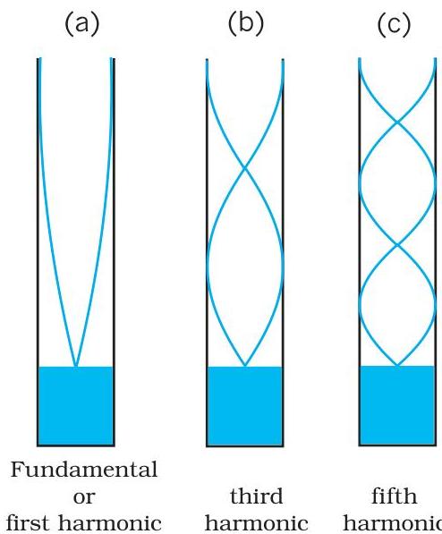
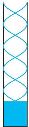
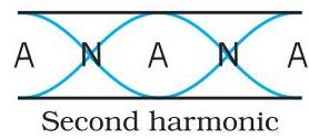
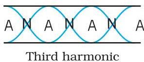
The lowest natural frequency, or fundamental frequency, occurs when $n = 0$, and its value is $\frac{v}{4L}$. Frequencies exceeding this fundamental are categorised as odd harmonics, meaning they are odd integer multiples of the fundamental frequency, such as $3\frac{v}{4L}$, $5\frac{v}{4L}$, and so forth. Figure 14.14 illustrates the initial six odd harmonics for an air column that is closed at one end and open at the other. In the case of a pipe open at both ends, each opening functions as an antinode. It is readily apparent that an air column open at both extremities produces a complete set of harmonics (Refer to Fig. 14.15).
The aforementioned systems, including strings and air columns, are also capable of exhibiting forced oscillations (as discussed in Chapter 13). Should an external driving frequency closely approximate one of the system's inherent natural frequencies, the phenomenon of resonance will be observed.
For a circular membrane, such as that found on a tabla, which is firmly secured around its perimeter, the normal modes are dictated by the boundary condition stipulating that no portion of the membrane's circumference undergoes vibration. Calculating the frequencies of the normal modes for such a system presents a greater degree of complexity. This particular challenge entails the analysis of wave propagation across two dimensions. Nonetheless, the fundamental physical principles remain consistent.
Example 14.5 Consider a pipe with a length of $30.0\mathrm{cm}$, open at both ends. Which specific harmonic mode of this pipe would resonate with a $1.1\mathrm{kHz}$ source? Furthermore, if one end of the pipe were subsequently closed, would resonance still occur with the identical source? Assume the speed of sound in air to be $330\mathrm{ms}^{-1}$.
Answer The frequency of the first harmonic is determined by:
$ v _ {1} = \frac {v}{\lambda_ {1}} = \frac {v}{2 L} \quad (\text { open pipe}) $
where $L$ denotes the pipe's length. The frequency corresponding to its $n$-th harmonic is:
$ v _ {n} = \frac {n v}{2 L}, \text { for } n = 1, 2, 3, \dots (\text { open pipe}) $
Figure 14.15 illustrates the initial several modes for an open pipe.
Considering $L = 30.0\mathrm{cm}$ and $v = 330\mathrm{ms}^{-1}$,
$ v _ {n} = \frac {n 3 3 0 (m s ^ {- 1})}{0 . 6 (m)} = 5 5 0 n s ^ {- 1} $
Evidently, a $1.1\mathrm{kHz}$ frequency source will induce resonance at $\nu_{2}$, which corresponds to the second harmonic.
WAVES
 (d)
seventh harmonic
Fig. 14.14 Illustrative representations of the characteristic vibrational patterns (normal modes) within an air column that is open at one extremity and sealed at the other. It is evident that only the odd-numbered harmonics are permissible under these conditions.
(d)
seventh harmonic
Fig. 14.14 Illustrative representations of the characteristic vibrational patterns (normal modes) within an air column that is open at one extremity and sealed at the other. It is evident that only the odd-numbered harmonics are permissible under these conditions.
 e
e
 (f)
ninth harmonic
eleventh harmonic
(f)
ninth harmonic
eleventh harmonic
Considering a scenario where one end of the pipe is sealed (as depicted in Fig. 14.15), the fundamental frequency can be ascertained from Eq. (14.15) as:
$ v _ {I} = \frac {v}{\lambda_ {1}} - \frac {v}{4 L} \text {(pipe closed at one end)} $
Furthermore, only the harmonics characterised by odd numbers are observed:
$ v _ {3} = \frac {3 v}{4 L}, v _ {3} = \frac {5 v}{4 L}, \text { and so on. } $
Given a pipe length L of 30 cm and a wave speed $\nu$ of $330 , \text{m} , \text{s}^{-1}$, the fundamental frequency for a pipe closed at one end is calculated to be $275 , \text{Hz}$. If the source frequency aligns with the fourth harmonic of this system, no resonance phenomenon will manifest with the source upon the closure of one end, as the fourth harmonic does not constitute an allowed vibrational mode.
14.7 BEATS
The phenomenon known as 'beats' represents an intriguing outcome of wave interference. When two harmonic sound waves possessing slightly differing, yet proximate, frequencies are simultaneously perceived, the listener detects a sound whose primary frequency is the average of the two constituent frequencies. Crucially, an additional auditory characteristic emerges: a perceptibly distinct periodic fluctuation in the sound's intensity, occurring at a frequency equivalent to the absolute difference between the two original frequencies. This effect finds common practical application among musicians,
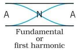 Fig. 14.15 Standing waves in an open pipe, first four harmonics are depicted.
who utilise it to synchronise their instruments. The tuning process continues until their acutely trained ears no longer discern any beats.
For a mathematical exposition of this phenomenon, let us analyse two harmonic sound waves characterised by nearly identical angular frequencies, $\omega_{1}$ and $\omega_{2}$. For analytical simplicity, we shall fix the observation point at $x = 0$. By referencing Eq. (14.2), and making an appropriate selection of phase (specifically, $\phi = \pi /2$ for each wave), alongside the assumption of equal amplitudes, we can express these waves as:
$s_{1} = a\cos \omega_{1}t$ and $s_2 = a\cos \omega_2t$ (14.45)
Here, the symbol $y$ has been substituted with $s$, signifying that we are addressing longitudinal displacement rather than transverse displacement. Let us designate $\omega_{1}$ as the marginally higher of the two frequencies. According to the principle of superposition, the resultant displacement is given by:
$ s = s _ {1} + s _ {2} = a (\cos \omega_ {1} t + \cos \omega_ {2} t) $
Applying the well-known trigonometric identity for $\cos A + \cos B$, we derive:
$ = 2 a \cos \frac {\left(\omega_ {1} - \omega_ {2}\right) t}{2} \cos \frac {\left(\omega_ {1} + \omega_ {2}\right) t}{2} \tag {14.46} $
This expression can be alternatively represented as:
$ s = \left[ 2 a \cos \omega_ {b} t \right] \cos \omega_ {a} t \tag {14.47} $
where
$ \omega_ {b} = \frac {\left(\omega_ {1} - \omega_ {2}\right)}{2} \text { and } \omega_ {a} = \frac {\left(\omega_ {1} + \omega_ {2}\right)}{2} $
If we now consider the condition where the absolute difference in angular frequencies, $|\omega_1 - \omega_2|$, is significantly smaller than $\omega_1$ (which inherently implies that $\omega_{a}$ is much greater than $\omega_{b}$), Eq. (14.47) can be interpreted as follows. The composite wave oscillates at the average angular frequency, $\omega_{a}$. However, its amplitude is not constant over time, distinguishing it from a pure harmonic wave. The amplitude reaches its peak magnitude when the term $\cos \omega_{b}t$ attains its extreme values of $+1$ or $-1$. Consequently, the intensity of the resulting wave undergoes periodic increases and decreases (waxing and waning) with a frequency defined as $2\omega_{b} = \omega_{1} - \omega_{2}$.

Musical Pillars
While many temple columns depict musicians, it is rare for the pillars themselves to generate sound. However, at the Nellaiappar temple in Tamil Nadu, a gentle percussive touch on a group of columns, each sculpted from a monolithic rock, elicits the fundamental notes of Indian classical music: Sa, Re, Ga, Ma, Pa, Dha, Ni, Sa. The resonant properties of these pillars are governed by the stone's elasticity, its material density, and its structural form.
These sonorous pillars are classified into three distinct categories. The first, known as the Shruti Pillar, is capable of producing the foundational musical notes, or "swaras." The second type, termed Gana Thoongal, creates the elementary melodies that constitute "ragas." The third classification, Laya Thoongal pillars, generates "taal" (rhythmic beats) upon impact. The pillars found at the Nellaiappar temple exhibit characteristics of both the Shruti and Laya varieties.
Archaeological evidence places the construction of the Nellaiappar temple in the 7th century, attributing its development to a series of rulers from the Pandyan dynasty.
The melodic pillars at Nellaiappar, alongside those in various other South Indian temples such as Hampi (picture), Kanyakumari, and Thiruvananthapuram, represent an architectural and acoustic phenomenon exclusive to this nation, without precedent elsewhere globally.
$\omega_{2}$ . Since $\omega = 2\pi \nu$ , the beat frequency $\nu_{beat}$ , is given by
$ v _ {\text {b e a t}} = v _ {1} - v _ {2} \tag {14.48} $
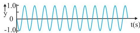
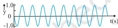
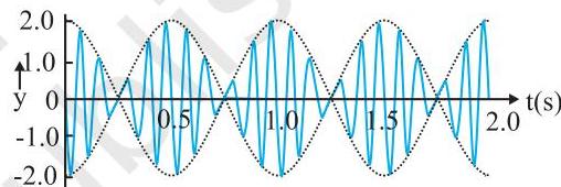
Fig. 14.16 visually demonstrates the beat phenomenon resulting from the superposition of two harmonic waves with frequencies of 11 Hz and 9 Hz. The amplitude of the composite wave exhibits beats at a frequency of 2 Hz.
 (a)
(a)
 (b)
(b)
 (c)
Fig. 14.16 Depicting the superposition of two harmonic waves: one with a frequency of $11\mathrm{Hz}$ (a), and another with a frequency of $9\mathrm{Hz}$ (b), resulting in beats with a frequency of $2\mathrm{Hz}$ , as illustrated in (c).
(c)
Fig. 14.16 Depicting the superposition of two harmonic waves: one with a frequency of $11\mathrm{Hz}$ (a), and another with a frequency of $9\mathrm{Hz}$ (b), resulting in beats with a frequency of $2\mathrm{Hz}$ , as illustrated in (c).
Example 14.6 Two sitar strings, A and B, when playing the 'Dha' note, are slightly dissonant, generating a beat frequency of $5\mathrm{Hz}$ . When the tension in string B is marginally increased, the beat frequency is observed to reduce to $3\mathrm{Hz}$ . Determine the initial frequency of string B, given that the frequency of string A is $427\mathrm{Hz}$ ?
Answer An augmentation in the tension applied to a string leads to a rise in its frequency. Had the initial frequency of string $\mathrm{B}(\nu_{B})$ exceeded that of string $\mathrm{A}(\nu_{A})$ , a subsequent increment in $\nu_{B}$ would logically have caused an escalation in the beat frequency. However, the observed beat frequency diminishes. This observation indicates that $\nu_{B} < \nu_{A}$ . Given that $\nu_{A} - \nu_{B} = 5\mathrm{Hz}$ and $\nu_{A} = 427\mathrm{Hz}$ , we deduce that $\nu_{B} = 422\mathrm{Hz}$ .
SUMMARY
Newton's Laws dictate the behavior of mechanical waves, which necessitate a material medium for their propagation.
In transverse waves, the oscillations of the medium's particles occur perpendicularly to the path of wave propagation.
Conversely, longitudinal waves are characterised by the oscillation of medium particles in the same direction as the wave's propagation.
A progressive wave is defined as a disturbance that travels through a medium, transferring energy from one location to another.
For a sinusoidal wave propagating along the positive $x$-axis, its displacement can be mathematically expressed as:
$ y (x, t) = a \sin (k x - \omega t + \phi) $
Here, $a$ represents the wave's amplitude, $k$ denotes the angular wave number, $\omega$ signifies the angular frequency, the term $(kx - \omega t + \phi)$ constitutes the phase, and $\phi$ is identified as the phase constant or initial phase angle.
The wavelength ($\lambda$) of a progressive wave is defined as the spatial separation between two successive points that are in the identical phase at any specific instant. For a stationary wave, this quantity corresponds to twice the separation between two adjacent nodes or antinodes.
The period ($T$) of a wave's oscillation is characterised as the duration required for any given element within the medium to complete one full oscillatory cycle. This period is mathematically linked to the angular frequency ($\omega$) by the following relationship:
$ T = \frac {2 \pi}{\omega} $
The frequency ($\nu$) of a wave is established as the reciprocal of its period ($1/T$) and can also be expressed in terms of angular frequency as:
$ \nu = \frac {\omega}{2 \pi} $
The propagation speed ($v$) of a progressive wave can be determined by the expressions $v = \frac{\omega}{k} = \frac{\lambda}{T} = \lambda v$.
For a transverse wave propagating along a stretched string, its speed is intrinsically defined by the string's inherent characteristics. Specifically, the velocity ($v$) on such a string, possessing tension $T$ and linear mass density $\mu$, is given by:
$ v = \sqrt {\frac {T}{\mu}} $
Sound waves represent longitudinal mechanical disturbances capable of propagating through solid, liquid, or gaseous media. The velocity ($v$) of a sound wave within a fluid, characterised by its bulk modulus $B$ and density $\rho$, is expressed as:
$ v = \sqrt {\frac {B}{\rho}} $
Furthermore, the speed of longitudinal waves within a metallic bar is determined by:
$ v = \sqrt {\frac {Y}{\rho}} $
In the case of gases, given the relationship $B = \gamma P$, the speed of sound can be calculated as:
$ v = \sqrt {\frac {\gamma P}{\rho}} $
Should multiple waves propagate concurrently within the same medium, the resultant displacement of any constituent element of that medium is equivalent to the algebraic summation of the individual displacements caused by each wave. This fundamental concept is termed the principle of superposition of waves:
$ y = \sum_{i=1}^{n} f_i(x - vt) $
When two sinusoidal waves coexist on the same string, they manifest interference phenomena, either reinforcing or attenuating each other in accordance with the principle of superposition. If these two waves are travelling in the identical direction, possess identical amplitude $a$ and frequency, but are phase-shifted by a constant $\phi$, the outcome is a singular wave maintaining the same frequency $\omega$:
$ y(x, t) = \left[ 2a\cos \frac{1}{2}\phi \right] \sin \left(kx - \omega t + \frac{1}{2}\phi\right) $
Specifically, if $\phi$ equals $0$ or any integer multiple of $2\pi$, the waves are precisely in phase, leading to constructive interference; conversely, if $\phi$ is $\pi$, they are precisely out of phase, resulting in destructive interference.
When a propagating wave encounters a rigid boundary or a closed termination, it undergoes reflection accompanied by a phase inversion. Conversely, reflection occurring at an open boundary proceeds without any alteration in its phase.
For an incident wave
$ y_r(x, t) = a \sin (kx - \omega t) $
the reflected wave at a rigid boundary is
$ y_r(x, t) = -a \sin (kx + \omega t) $
For reflection at an open boundary
$ y_r(x, t) = a \sin (kx + \omega t) $
- Standing waves are generated through the superposition of two identical waves propagating in contrary directions. In the case of a string constrained at both extremities, the mathematical expression for a standing wave is provided by:
$ y(x, t) = \left[ 2a \sin kx \right] \cos \omega t $
Standing wave patterns are distinguished by stationary points of zero displacement, termed nodes, and fixed points of maximal displacement, referred to as antinodes. The spatial distance between any two successive nodes or antinodes is $\frac{\lambda}{2}$.
A taut string of length $L$, secured at both its termini, exhibits vibrational modes corresponding to frequencies specified by:
$ v = \frac{nv}{2L}, \quad n = 1, 2, 3, \dots $
These frequencies, derived from the aforementioned relationship, constitute the system's normal modes of oscillation. The mode of oscillation possessing the lowest frequency is identified as the fundamental mode or the first harmonic. Subsequent harmonics correspond to increasing values of $n$, such as the second harmonic for $n = 2$, and so forth.
For a pipe of length $L$ that is closed at one end and open at the other (e.g., air columns), the frequencies at which it resonates are determined by:
$ v = (n + \frac{1}{2}) \frac{v}{2L}, \quad n = 0, 1, 2, 3, \dots $
The frequencies described by this relation represent the normal modes of oscillation for such a configuration. The minimum frequency, expressed as $v / 4L$, corresponds to the fundamental mode or the first harmonic.
Systems like a string of length $L$ secured at both extremities, or an air column either closed at one end and open at the other, or open at both ends, oscillate at specific characteristic frequencies known as their normal modes. Every one of these normal mode frequencies also functions as a resonant frequency for the respective system.
Beats are phenomena that manifest when two waves possessing marginally dissimilar frequencies, $\nu_1$ and $\nu_2$, along with comparable amplitudes, are superimposed. The resulting beat frequency is calculated as:
$ \nu_{beat} = \nu_1 - \nu_2 $
| Physical quantity | Symbol | Dimensions | Unit | Remarks |
|---|---|---|---|---|
| Wavelength | λ | [L] | m | Distance between two consecutive points with the same phase. |
| Propagation constant | k | [L^{-1}] | m^{-1} | $k = \frac{2\pi}{\lambda}$ |
| Wave speed | v | [LT^{-1}] | m s^{-1} | $v = \nu\lambda$ |
| Beat frequency | $\nu_{beat}$ | [T^{-1}] | s^{-1} | Difference of two close frequencies of superposing waves. |
POINTS TO PONDER
- A wave does not represent the bulk movement of matter within a medium. For instance, wind, which involves the displacement of air from one location to another, is distinct from a sound wave in air, which is characterised by localised compressions and rarefactions of air layers.
- In wave propagation, it is energy, rather than matter, that is transported from one point to another.
- The transfer of energy in a mechanical wave occurs through the elastic coupling forces present between adjacent oscillating components of the medium.
- Transverse waves can only propagate in media possessing a shear modulus of elasticity. Longitudinal waves, conversely, require a bulk modulus of elasticity, which enables their propagation through all phases of matter, including solids, liquids, and gases.
- In a harmonic progressive wave of a specified frequency, all particles exhibit the same amplitude but possess varying phases at any given instant. In contrast, within a stationary wave, all particles situated between two consecutive nodes share an identical phase at a specific moment, yet they display different amplitudes.
- For an observer at rest within a medium, the speed (v) of a mechanical wave in that medium is exclusively determined by the medium's elastic and other properties (such as its mass density). It is not influenced by the velocity of the wave source.
EXERCISES
14.1 A string possessing a mass of $2.50,\mathrm{kg}$ is subjected to a tension of $200,\mathrm{N}$. The length of this extended string measures $20.0,\mathrm{m}$. If a transverse perturbation is initiated at one extremity of the string, what duration is required for this disturbance to propagate to the opposing end?
14.2 A stone is released from the summit of a tower with a height of $300,\mathrm{m}$, subsequently plunging into a body of water situated at the tower's base. At what moment is the sound of the splash perceived at the tower's top, given that the speed of sound in air is $340,\mathrm{m,s^{-1}}$? (Assume $g = 9.8,\mathrm{m,s^{-2}}$)
14.3 A steel wire exhibits a length of $12.0,\mathrm{m}$ and a mass of $2.10,\mathrm{kg}$. What magnitude of tension must be applied to this wire for the velocity of a transverse wave travelling along it to equal the speed of sound in dry air at $20^{\circ}\mathrm{C}$, which is $343,\mathrm{m,s^{-1}}$?
14.4 Utilise the equation $v = \sqrt{\frac{\gamma P}{\rho}}$ to elucidate why the speed of sound in air:
(a) remains unaffected by changes in pressure, (b) exhibits an increase as temperature rises, (c) shows an increment with heightened humidity.
14.5 It has been established that a one-dimensional travelling wave can be described by a function $y = f(x, t)$, where the spatial variable $x$ and the temporal variable $t$ invariably appear combined as either $x - vt$ or $x + vt$, i.e., $y = f(x \pm vt)$. Is the inverse of this statement also valid? Investigate whether the following functions for $y$ could potentially represent a travelling wave:
(a) $(x - vt)^2$ (b) $\log [(x + vt) / x_0]$ (c) $1 / (x + vt)$
14.6 A bat emits ultrasonic sound waves with a frequency of $1000,\mathrm{kHz}$ into the air. When these sound waves encounter a water surface, determine the wavelength of (a) the reflected sound, and (b) the transmitted sound. The speed of sound in air is $340,\mathrm{m,s^{-1}}$ and in water is $1486,\mathrm{m,s^{-1}}$.
14.7 A medical institution employs an ultrasonic scanner to pinpoint tumours within biological tissue. Given that the speed of sound within this tissue is $1.7,\mathrm{km,s^{-1}}$ and the scanner's operational frequency is $4.2,\mathrm{MHz}$, what is the corresponding wavelength of the sound in the tissue?
14.8 A transverse harmonic wave propagating on a string is mathematically expressed as:
$ y (x, t) = 3.0 \sin (36 t + 0.018 x + \pi / 4) $
where $x$ and $y$ are quantified in centimetres and $t$ in seconds. The positive direction for $x$ is defined from left to right.
(a) Is this wave categorised as a travelling wave or a stationary wave? If it is a travelling wave, determine its propagation speed and direction.
(b) What are its amplitude and its oscillation frequency? (c) What is the initial phase at the origin ($x=0, t=0$)? (d) What constitutes the smallest spatial separation between two consecutive crests within this wave?
14.9 For the wave detailed in Exercise 14.8, generate graphs depicting the displacement $(y)$ versus time $(t)$ for the spatial locations $x = 0,\mathrm{cm}$, $x = 2,\mathrm{cm}$, and $x = 4,\mathrm{cm}$. Characterise the geometric forms of these graphs. Furthermore, specify which attributes of the oscillatory motion in a travelling wave—amplitude, frequency, or phase—exhibit variation from one point to another in space.
14.10 Considering the travelling harmonic wave given by:
$ y (x, t) = 2.0 \cos 2 \pi (10 t - 0.0080 x + 0.35) $
where $x$ and $y$ are expressed in centimetres and $t$ in seconds. Calculate the phase difference between the oscillatory motions of two points separated by the following distances:
(a) $4,\mathrm{m}$ (b) $0.5,\mathrm{m}$ (c) $\lambda /2$ (d) $3\lambda /4$
14.11 For a string fixed at both extremities, its transverse displacement is described by the relation:
$ y (x, t) = 0.06 \sin \left(\frac {2 \pi}{3} x\right) \cos (120 \pi t) $
Here, $x$ and $y$ are expressed in metres, and $t$ in seconds. The string possesses a length of $1.5\mathrm{m}$ and a mass of $3.0\times 10^{-2}\mathrm{kg}$.
Answer the following :
(a) Does this mathematical expression characterise a propagating wave or a standing wave? (b) Deconstruct this wave into a superposition of two distinct waves moving in contrary directions. Determine the wavelength, frequency, and propagation speed for each of these constituent
waves. (c) Calculate the tensile force present in the string.
14.12 (i) Considering the wave phenomenon on the string detailed in Exercise 15.11, do all locations along the string undergo oscillation with identical (a) frequency, (b) phase, (c) amplitude? Provide justifications for your responses. (ii) What is the oscillation amplitude at a position situated 0.375 m from one of its termini?
14.13 Presented below are several functions of $x$ and $t$, each intended to model the displacement (either transverse or longitudinal) of an elastic wave. Identify which of these correspond to (i) a propagating wave, (ii) a standing wave, or (iii) neither of these classifications:
(a) $y = 2\cos (3x)\sin (10t)$ (b) $y = 2\sqrt{x - vt}$ (c) $y = 3\sin (5x - 0.5t) + 4\cos (5x - 0.5t)$ (d) $y = \cos x\sin t + \cos 2x\sin 2t$
14.14 A string held taut between two fixed anchor points oscillates in its primary vibrational mode at a frequency of 45 Hz. The string's total mass is $3.5 \times 10^{-2} , \mathrm{kg}$, and its linear mass density is $4.0 \times 10^{-2} , \mathrm{kg} , \mathrm{m}^{-1}$. Determine (a) the propagation velocity of a transverse wave along this string, and (b) the tensile force exerted within the string.
14.15 A tube measuring one metre in length, open at one extremity and fitted with an adjustable piston at the opposite end, exhibits resonance when exposed to a constant frequency source (specifically, a tuning fork operating at 340 Hz). This resonant condition occurs when the effective tube length is either 25.5 cm or 79.3 cm. Based on this, calculate the approximate speed of sound in the ambient air during the experimental procedure. Disregard any end corrections.
14.16 A steel cylindrical rod, 100 cm in length, is securely fastened at its midpoint. The fundamental frequency for the longitudinal oscillations of this rod is provided as 2.53 kHz. What is the velocity of sound propagation through steel under these conditions?
14.17 A cylindrical pipe, 20 cm in length, is sealed at one end. Which specific harmonic mode of this pipe is stimulated into resonance by a sound source emitting 430 Hz? Would the identical sound source achieve resonance with the pipe if both of its ends were open? (Assume the speed of sound in air is 340 m s⁻¹).
14.18 Two strings from a sitar, designated A and B, when played to produce the note 'Ga', are slightly detuned, resulting in an audible beat frequency of 6 Hz. Subsequently, the tension applied to string A is marginally decreased, causing the beat frequency to diminish to 3 Hz. Given that the initial frequency of string A was 324 Hz, what is the frequency of string B?
14.19 Explain why (or how):
(a) in the context of a sound wave, a point of zero displacement amplitude corresponds to a point of maximum pressure variation, and conversely, (b) bats possess the capability to determine the range, orientation, composition, and dimensions of obstructions in their environment without relying on visual perception, (c) despite sharing an identical fundamental frequency, a musical note produced by a violin and one by a sitar are perceptibly distinguishable, (d) solid materials are capable of sustaining both longitudinal and transverse wave propagation, whereas gaseous media exclusively permit the transmission of longitudinal waves, and (e) a wave packet undergoes deformation of its characteristic profile as it traverses through a medium exhibiting dispersion.