System of Particles and Rotational Motion - CBSE Class 11 Physics Notes

CHAPTER SIX

SYSTEMS OF PARTICLES AND ROTATIONAL MOTION

6.1 Introduction
6.2 Centre of mass
6.3 Motion of centre of mass
6.4 Linear momentum of a system of particles
6.5 Vector product of two vectors
6.6 Angular velocity and its relation with linear velocity
6.7 Torque and angular momentum
6.8 Equilibrium of a rigid body
6.9 Moment of inertia
6.10 Kinematics of rotational motion about a fixed axis
6.11 Dynamics of rotational motion about a fixed axis
6.12 Angular momentum in case of rotation about a fixed axis

Summary
Points to Ponder
Exercises

6.1 INTRODUCTION

Our previous analyses predominantly focused on the dynamics of individual particles. (Conceptually, a particle is modeled as a dimensionless point mass.) The insights gained from these studies were extended to encompass the movement of objects possessing finite dimensions, based on the premise that such motion could be characterized by that of a single particle.

Conversely, all physical objects encountered in everyday experience possess finite dimensions. When examining the kinematics and dynamics of extended bodies—those with measurable size—the simplified particle model frequently proves insufficient. This chapter aims to transcend this limitation by developing a comprehensive framework for understanding the behavior of extended bodies. Fundamentally, an extended body can be conceptualized as an assembly of particles. Our initial focus will be on the collective motion of such systems. A pivotal concept in this endeavor will be the center of mass of a particle system. We will explore the motion of this center of mass and its utility in elucidating the dynamics of extended bodies.

Many challenges associated with extended bodies become tractable by modeling them as rigid bodies. Conceptually, a rigid body is defined as an entity maintaining an absolutely fixed and immutable form, where the spatial separation between any two constituent particles remains constant. This definition inherently implies that no actual physical object is perfectly rigid, as all real materials exhibit deformation when subjected to external forces. Nevertheless, in numerous practical scenarios, these deformations are inconsequential. Consequently, for a variety of objects, including wheels, gyroscopes, structural beams, molecular structures, and celestial bodies, their warping, bending, or vibrational tendencies can often be disregarded, allowing them to be analyzed as rigid systems.

6.1.1 What kind of motion can a rigid body have?

To investigate this query, let us consider various instances of rigid body movement. We shall commence with a rectangular block.

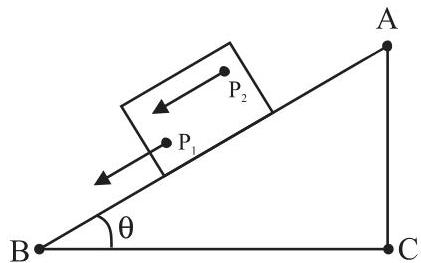Fig 6.1 Translational (sliding) motion of a block down an inclined plane.

(Any point on the block, such as $P_{1}$ or $P_{2}$, maintains an identical velocity at every instant.)

The block slides down an inclined plane without any lateral displacement. This block is treated as a rigid body. Its descent along the plane is characterized by all its constituent particles moving in unison, signifying they possess the same velocity at any given moment. In this scenario, the rigid body exhibits pure translational motion (Fig. 6.1).

At any specific instant in pure translational motion, all particles within the body share the same velocity.

Now, let us examine the rolling motion of a solid metallic or wooden cylinder down the identical inclined plane (Fig. 6.2). The rigid body in question, the cylinder, progresses from the top to the bottom of the inclined plane, thereby appearing to undergo translational motion. However, as depicted in Fig. 6.2, its particles do not all possess the same velocity simultaneously. Consequently, the body is not engaged in pure translational motion; its movement comprises translation augmented by an additional component.

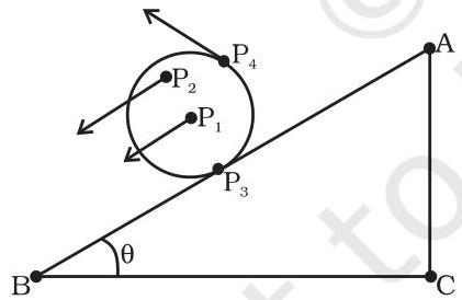Fig. 6.2 Rolling motion of a cylinder. It is not pure translational motion. Points $P_{1}, P_{2}, P_{3}$ and $P_{4}$ exhibit distinct velocities (indicated by arrows) at any given instant. Notably, the velocity of the contact point $P_{2}$ is zero at any instant if the cylinder rolls without slipping.

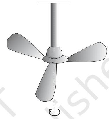
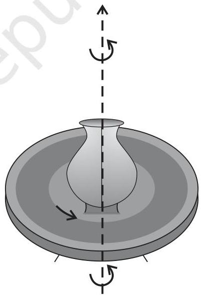
To comprehend this "additional component," let us consider a rigid body whose movement is restricted such that it cannot undergo translation. The most typical method to constrain a rigid body against translational motion involves fixing it along a straight line. The sole permissible motion for such a rigid body is rotation. The line, or fixed axis, around which the body rotates is termed its axis of rotation. Observing our surroundings, numerous examples of rotation about an axis can be found, including a ceiling fan, a potter's wheel, a giant wheel at a fair, a merry-go-round, and so forth (Fig 6.3(a) and (b)).

(a)

(b) Fig. 6.3 Rotation about a fixed axis

(a) A ceiling fan (b) A potter's wheel.

Let us endeavor to grasp the nature of rotation and its defining characteristics. It can be observed that during the rotation of a rigid body about a fixed axis,

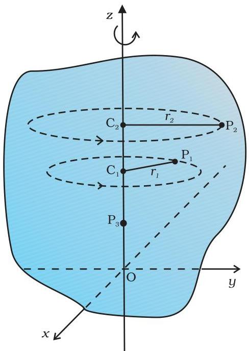Fig. 6.4 A rigid body rotation about the $z$-axis (Each point of the body, such as $P_{1}$ or $P_{2}$, traces a circular path with its center ($C_{1}$ or $C_{2}$) located on the axis of rotation. The radius of this circle ($r_{1}$ or $r_{2}$) corresponds to the perpendicular distance from the point ($P_{1}$ or $P_{2}$) to the axis. A point situated directly on the axis, like $P_{2}$, remains stationary).

Within a rigid body undergoing rotation about a fixed axis, each constituent particle traces a circular path. This circular trajectory resides in a plane orthogonal to the axis, with its center situated directly on the axis. As illustrated in Fig. 6.4, consider the rotational dynamics of a rigid body around a stationary axis, specifically the $z$ -axis within the chosen reference frame. If we select an arbitrary particle, $\mathrm{P}_1$, within this rigid body, located at a radial distance $r_1$ from the fixed axis, it will execute motion along a circle of radius $r_1$. The center of this circle, $\mathrm{C}_1$, lies on the fixed axis, and the plane containing this circle is perpendicular to the axis. Similarly, another particle, $\mathrm{P}_2$, positioned at a distance $r_2$ from the fixed axis, will also follow a circular path of radius $r_2$, with its center $\mathrm{C}_2$ on the axis. This latter circle also occupies a plane perpendicular to the axis. It is important to note that while the circular paths of $\mathrm{P}_1$ and $\mathrm{P}_2$ may occupy distinct planes, both these planes invariably maintain an orthogonal relationship with the fixed axis. Conversely, any particle, such as $\mathrm{P}_3$, located directly on the axis itself, where $r = 0$, will remain motionless during the body's rotation. This static behavior is a direct consequence of the axis of rotation being fixed.

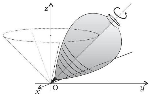Fig. 6.5 (a) A spinning top (The point of contact of the top with the ground, its tip $O$, is fixed.)

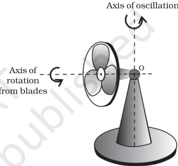Fig. 6.5 (b) An oscillating table fan with rotating blades. The pivot of the fan, point $O$, is fixed. The blades of the fan are under rotational motion, whereas, the axis of rotation of the fan blades is oscillating.

However, certain instances of rotational motion involve an axis that is not stationary. A notable illustration of this phenomenon is a top that spins in a fixed location [Fig. 6.5(a)]. (For this discussion, we postulate that the top does not undergo translation, thus lacking any linear motion.) Empirical observation reveals that the rotational axis of such a spinning top describes a conical path around the vertical line passing through its point of contact with the ground, as depicted in Fig. 6.5(a). (This characteristic movement of the top's axis about the vertical is referred to as precession.) It is crucial to observe that the point where the top touches the ground remains fixed. At any given moment, the top's axis of rotation invariably extends through this fixed point of contact. An additional straightforward example of this rotational category is an oscillating table fan or a pedestal fan [Fig. 6.5(b)]. One might have noticed that the

SYSTEMS OF PARTICLES AND ROTATIONAL MOTION

rotational axis of such a fan exhibits an oscillatory (lateral) displacement within a horizontal plane, centered around the vertical line that intersects the pivot point (designated as point O in Fig. 6.5(b)).

Even as the fan rotates and its axis undergoes lateral movement, this specific pivot point remains stationary. Consequently, in more comprehensive scenarios of rotation, exemplified by a spinning top or a pedestal fan, it is a singular point, rather than an entire line, within the rigid body that maintains a fixed position. Although the axis itself is not fixed in these instances, it consistently traverses through this stationary point. Nevertheless, for the purposes of this particular study, our primary focus will be directed towards the more straightforward and specific case of rotation where a single line (i.e., the axis) is rigidly fixed.

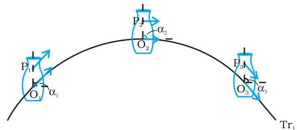Fig. 6.6(a) Motion of a rigid body which is pure translation.

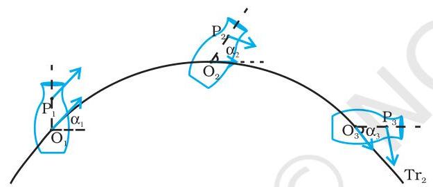Fig. 6.6(b) Motion of a rigid body which is a combination of translation and rotation.

Figures 6.6(a) and 6.6(b) depict distinct modes of motion for an identical rigid body. Let $P$ denote an arbitrary point within the body, and $O$ represent its center of mass—a concept elucidated in the subsequent section. For our current discussion, it is sufficient to understand that the paths traversed by $O$ correspond to the body's translational trajectories, designated as $Tr_{1}$ and $Tr_{2}$. The locations of points $O$ and $P$ at three successive moments are indicated by $O_{1}, O_{2}, O_{3}$ and $P_{1}, P_{2}, P_{3}$ respectively, across both illustrations. In the context of pure translational motion, as shown in Fig. 6.6(a), the velocities of any two points on the body, such as $O$ and $P$, are identical at any given instant. Furthermore, the alignment of the segment $OP$—specifically, the angle it forms with a constant reference direction, such as the horizontal—is invariant, meaning $\alpha_{1} = \alpha_{2} = \alpha_{3}$. Conversely, Fig. 6.6(b) presents a scenario involving both translational and rotational motion. Here, the instantaneous velocities of $O$ and $P$ are not necessarily equal, and the angles $\alpha_{1}, \alpha_{2},$ and $\alpha_{3}$ can exhibit variations.

Consequently, within this discussion, rotational motion will be considered exclusively about a fixed axis, unless an alternative condition is explicitly specified.

The phenomenon of a cylinder rolling down an inclined plane exemplifies a combined motion, integrating rotation around a fixed axis with translation. Therefore, the additional component of motion previously alluded to in the context of rolling is identified as rotational motion. Figures 6.6(a) and (b) offer valuable insights into this distinction. Both illustrations depict the movement of an identical body following the same translational path. In the instance of Fig. 6.6(a), the motion is purely translational; conversely, in Fig. 6.6(b), it constitutes a blend of translation and rotation. (Readers are encouraged to replicate these two distinct motion types using a rigid object, such as a substantial book.)

To summarize the principal insights derived from this section: A rigid body not constrained by pivoting or fixation exhibits motion that is either exclusively translational or a composite of translation and rotation. Conversely, a rigid body that is pivoted or otherwise fixed is restricted to rotational motion. This rotation can occur around an axis that is stationary (as demonstrated by a ceiling fan) or around an axis that itself undergoes movement (for example, an oscillating table fan, as illustrated in Fig. 6.5(b)). For the scope of the current chapter, our analysis will be confined to rotational motion about a fixed axis.

6.2 CENTRE OF MASS

Our initial focus will be on defining the center of mass for a system of particles and subsequently exploring its importance. For clarity, we will commence with a two-particle arrangement, orienting the line connecting these particles along the $x$ -axis.

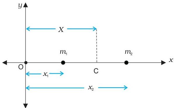Fig. 6.7

Consider two particles, with masses denoted as $m_{1}$ and $m_{2}$ respectively. Their respective positions, measured from a designated origin $O$, are $x_{1}$ and $x_{2}$. The system's center

of mass, labeled as point C, is situated at a distance $X$ from origin $O$, defined by the following expression:

$ X = \frac {m _ {1} x _ {1} + m _ {2} x _ {2}}{m _ {1} + m _ {2}} \tag {6.1} $

Equation (6.1) illustrates $X$ as the weighted average of $x_{1}$ and $x_{2}$, with the masses serving as the weighting factors. Should both particles possess identical mass, i.e., $m_{1} = m_{2} = m$, then the relationship simplifies to:

$ X = \frac {m x _ {1} + m x _ {2}}{2 m} = \frac {x _ {1} + x _ {2}}{2} $

Consequently, when two particles share an identical mass, their center of mass is positioned precisely at the midpoint of the line segment connecting them.

For a system comprising $n$ particles, each with masses $m_{1}, m_{2}, \ldots, m_{n}$ respectively, arranged along a straight line designated as the $x$-axis, the position of the system's center of mass is formally expressed as:

$ X = \frac {m _ {1} x _ {1} + m _ {2} x _ {2} + \dots + m _ {n} x _ {n}}{m _ {1} + m _ {2} + \dots + m _ {n}} = \frac {\sum_ {i = 1} ^ {n} m _ {i} x _ {i}}{\sum_ {i = 1} ^ {n} m _ {i}} = \frac {\sum_ {i} m _ {i} x _ {i}}{\sum_ {i} m _ {i}} \tag {6.2} $

Here, $x_{1}, x_{2}, \ldots, x_{n}$ represent the individual distances of each particle from the origin, and $X$ similarly denotes the center of mass position relative to the same origin. The Greek letter sigma, $\sum$, signifies a summation, specifically performed over all $n$ particles. The aggregate sum

$ \sum m _ {i} = M $

constitutes the total mass of the entire system.

Consider a scenario involving three particles that are not collinear. Within the plane containing these particles, we can establish $x-$ and $y-$ axes. The spatial locations of the three particles are then specified by coordinates $(x_{1},y_{1})$, $(x_{2},y_{2})$, and $(x_{3},y_{3})$, corresponding to their respective masses $m_{1}$, $m_{2}$, and $m_{3}$. The center of mass C for this three-particle system is consequently defined and positioned by the coordinates $(X,Y)$, which are determined by:

$ X = \frac {m _ {1} x _ {1} + m _ {2} x _ {2} + m _ {3} x _ {3}}{m _ {1} + m _ {2} + m _ {3}} \tag {6.3a} $

$ Y = \frac {m _ {1} y _ {1} + m _ {2} y _ {2} + m _ {3} y _ {3}}{m _ {1} + m _ {2} + m _ {3}} \tag {6.3b} $

In the specific instance where the particles possess equivalent masses, i.e., $m = m_{1} = m_{2} = m_{3}$, the equations become:

$ X = \frac {m (x _ {1} + x _ {2} + x _ {3})}{3 m} = \frac {x _ {1} + x _ {2} + x _ {3}}{3} $

$ Y = \frac {m (y _ {1} + y _ {2} + y _ {3})}{3 m} = \frac {y _ {1} + y _ {2} + y _ {3}}{3} $

Hence, when three particles share identical mass, their center of mass corresponds precisely to the geometric centroid of the triangular region defined by their positions.

The principles established in Equations (6.3a) and (6.3b) can be readily extended to encompass a system of $n$ particles that are spatially distributed and not restricted to a single plane. For such a configuration, the system's center of mass is located at the coordinates $(X, Y, Z)$, where

$ X = \frac {\sum m _ {i} x _ {i}}{M} \tag {6.4a} $

$ Y = \frac {\sum m _ {i} y _ {i}}{M} \tag {6.4b} $

$ \text{and} \quad Z = \frac {\sum m _ {i} z _ {i}}{M} \tag {6.4c} $

Here, $M = \sum m_{i}$ signifies the total mass of the system. The index $i$ iterates from 1 to $n$; $m_{i}$ denotes the mass of the $i^{\text{th}}$ particle, and its spatial location is specified by the coordinates $(x_{i}, y_{i}, z_{i})$.

The scalar expressions presented in Eqs. (6.4a), (6.4b), and (6.4c) can be consolidated into a single vector equation through the application of position vector formalism. We define $\mathbf{r}_i$ as the position vector corresponding to the $i$-th particle and $\mathbf{R}$ as the position vector delineating the center of mass:

$ \mathbf {r} _ {i} = x _ {i} \hat {\mathbf {i}} + y _ {i} \hat {\mathbf {j}} + z _ {i} \hat {\mathbf {k}} $

$ \text{and} \quad \mathbf {R} = X \hat {\mathbf {i}} + Y \hat {\mathbf {j}} + Z \hat {\mathbf {k}} $

Then, the combined vector equation is:

$ \mathbf {R} = \frac {\sum m _ {i} \mathbf {r} _ {i}}{M} \tag {6.4d} $

It is important to note that the summation appearing on the right-hand side of this expression represents a vector addition.

The utilization of vector notation significantly streamlines these expressions. A notable consequence arises if the origin of the chosen coordinate system coincides with the system's center of mass; in such a scenario, the vector sum $\sum m_{i}\mathbf{r}_{i}$ for the particle system evaluates to zero.

A rigid body, exemplified by objects like a meter stick or a flywheel, comprises a multitude of densely arranged particles. Consequently, the formulations provided in Eqs. (6.4a), (6.4b), (6.4c), and (6.4d) are equally pertinent to rigid bodies. However, the sheer quantity of constituent particles (atoms or molecules) within such a body renders direct summation over individual particles impractical. Given the minute inter-particle spacing, we are justified in modeling the body as a continuous mass distribution. To facilitate this, we conceptualize the body as being composed of $n$ infinitesimally

small mass elements, denoted as $\Delta m_{1}, \Delta m_{2}, \ldots, \Delta m_{n}$. Each $i$-th element, $\Delta m_{i}$, is considered to be situated at or around the point $(x_i, y_i, z_i)$. Under this approximation, the coordinates of the center of mass can be expressed as:

$ X = \frac {\sum (\Delta m _ {i}) x _ {i}}{\sum \Delta m _ {i}}, Y = \frac {\sum (\Delta m _ {i}) y _ {i}}{\sum \Delta m _ {i}}, Z = \frac {\sum (\Delta m _ {i}) z _ {i}}{\sum \Delta m _ {i}} $

As the number of elements $n$ approaches infinity and the magnitude of each $\Delta m_i$ approaches zero, these approximate expressions converge to their precise values. In this limit, the summations over $i$ are formally replaced by integrals. Specifically:

$ \sum \Delta m _ {i} \rightarrow \int \mathrm {d} m = M, $

$ \sum (\Delta m _ {i}) x _ {i} \rightarrow \int x \mathrm {d} m, $

$ \sum (\Delta m _ {i}) y _ {i} \rightarrow \int y \mathrm {d} m, $

and $\sum (\Delta m_{i})z_{i}\rightarrow \int z\mathrm{d}m$

In this context, $M$ signifies the total mass encompassing the entire body. The coordinates defining the center of mass are then precisely given by:

$ X = \frac {1}{M} \int x \mathrm {d} m, Y = \frac {1}{M} \int y \mathrm {d} m \text { and } Z = \frac {1}{M} \int z \mathrm {d} m \tag {6.5a} $

The unified vector representation corresponding to these three scalar components is given by:

$ \mathbf {R} = \frac {1}{M} \int \mathbf {r} \mathrm {d} m \tag {6.5b} $

When the center of mass is selected as the origin of a coordinate system, its position vector is defined as:

$ \mathbf {R} = \mathbf {0} $

This condition signifies that:

$ \mathrm {i . e .}, \int \mathbf {r} \mathrm {d} m = \mathbf {0} $

Which further implies that each component of the integral is zero:

$ \text {or} \int x \mathrm {d} m = \int y \mathrm {d} m = \int z \mathrm {d} m = 0 \tag {6.6} $

Frequently, the determination of the center of mass is required for homogeneous objects possessing regular geometries, such as rings, discs, spheres, or rods. (A homogeneous body is defined as one with a uniformly distributed mass.) Through the application of symmetry principles, it can be readily demonstrated that the centers of mass for these entities are situated at their respective geometric centers.

Fig. 6.8 Determining the CM of a thin rod.

Consider, for instance, a slender rod where its transverse dimensions (i.e., width and breadth for a rectangular cross-section, or radius for a cylindrical cross-section) are negligible compared to its longitudinal extent. If the origin is placed at the geometric center of the rod and the $x$-axis is aligned with its length, the principle of reflection symmetry dictates that for every mass element $dm$ positioned at $x$, an equivalent mass element $dm$ exists at $-x$ (refer to Fig. 6.8).

The cumulative contribution of each such pair to the integral, and consequently the integral $\int x\mathrm{d}m$ itself, sums to zero. As per Equation (6.6), the location where this integral evaluates to zero precisely defines the center of mass. Therefore, for a homogeneous thin rod, its center of mass is coincident with its geometric center. This phenomenon is attributable to reflection symmetry.

This identical argument based on symmetry is equally applicable to homogeneous rings, discs, spheres, and even more substantial rods with circular or rectangular cross-sections. In the case of all these bodies, it becomes apparent that for every infinitesimal mass element $dm$ situated at coordinates $(x, y, z)$, there invariably exists an identical mass element at the diametrically opposite point $(-x, -y, -z)$. (This signifies that the origin acts as a point of reflection symmetry for these configurations.) Consequently, all integrals presented in Equation (6.5 a) evaluate to zero. This implies that for all the aforementioned bodies, their center of mass corresponds precisely with their geometric center.

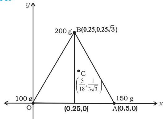
Example 6.1 Determine the center of mass for a system of three particles positioned at the vertices of an equilateral triangle. The masses of these particles are $100\mathrm{g}$, $150\mathrm{g}$, and $200\mathrm{g}$, respectively, and each side of the equilateral triangle measures $0.5\mathrm{m}$.

Answer Fig. 6.9

Adopting the coordinate system depicted in Fig. 6.9, the coordinates for the vertices O, A, and B of the equilateral triangle are established as (0,0), (0.5,0), and (0.25,0.25 $\sqrt{3}$), respectively. Assigning the masses $100\mathrm{g}$, $150\mathrm{g}$, and $200\mathrm{g}$ to positions O, A, and B, in that order, we can then calculate:

$ \begin{array}{l} X = \frac {m _ {1} x _ {1} + m _ {2} x _ {2} + m _ {3} x _ {3}}{m _ {1} + m _ {2} + m _ {3}} \ = \frac {1 0 0 (0) + 1 5 0 (0 . 5) + 2 0 0 (0 . 2 5) \mathrm {g m}}{(1 0 0 + 1 5 0 + 2 0 0) \mathrm {g}} \ = \frac {7 5 + 5 0}{4 5 0} \mathrm {m} = \frac {1 2 5}{4 5 0} \mathrm {m} = \frac {5}{1 8} \mathrm {m} \end{array} $

$ \begin{array}{l} Y = \frac {1 0 0 (0) + 1 5 0 (0) + 2 0 0 (0 . 2 5 \sqrt {3}) \mathrm {g m}}{4 5 0 \mathrm {g}} \ = \frac {5 0 \sqrt {3}}{4 5 0} \mathrm {m} = \frac {\sqrt {3}}{9} \mathrm {m} = \frac {1}{3 \sqrt {3}} \mathrm {m} \end{array} $

The center of mass C is depicted in the figure. Observe that it does not correspond to the geometric center of triangle OAB. What accounts for this distinction?

Example 6.2 Determine the center of mass of a triangular lamina.

Answer To determine this, the lamina $(\Delta LMN)$ can be conceptually segmented into slender strips, each oriented parallel to its base $(MN)$, as depicted in Fig. 6.10

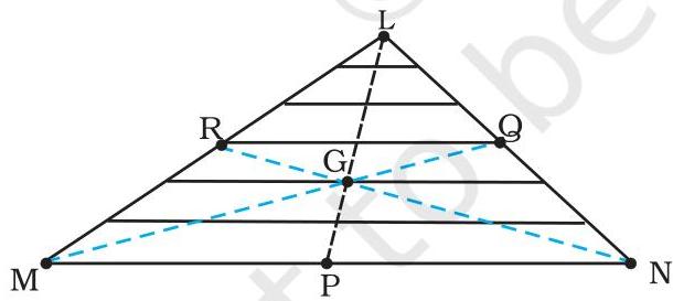Fig. 6.10

Due to symmetrical properties, the center of mass for each individual strip is situated at its midpoint. Connecting the midpoints of all such strips yields the median LP. Consequently, the center of mass for the entire triangular structure must reside along the median LP. Extending this reasoning, it can similarly be established that the center of mass also lies on medians MQ and NR. This implies that the center of mass is located at the intersection point of the medians, which is precisely the centroid (G) of the triangle.

Example 6.3 Ascertain the center of mass for a uniform L-shaped lamina (a slender planar sheet) with the specified dimensions. The total mass of this lamina is $3\mathrm{kg}$.

Answer By establishing the $X$ and $Y$ axes as depicted in Fig. 6.11, the coordinates corresponding to the vertices of the L-shaped lamina are provided within the illustration. One can conceptualize this L-shape as being composed of three individual squares, each possessing a side length of $1\mathrm{m}$. Given the uniform nature of the lamina, the mass of each square is $1\mathrm{kg}$. The centers of mass, designated $C_1$, $C_2$, and $C_3$, for these squares are, owing to symmetry, located at their respective geometric centers, with coordinates $(1/2, 1/2)$, $(3/2, 1/2)$, and $(1/2, 3/2)$ in sequence. For calculation purposes, the mass of each square is considered to be concentrated at these specific points. Consequently, the overall center of mass $(X, Y)$ for the entire L-shaped configuration is derived from the center of mass of these aggregated point masses.

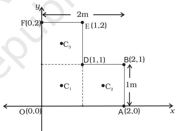Fig. 6.11

Therefore,

$ X = \frac {\left[ 1 (1 / 2) + 1 (3 / 2) + 1 (1 / 2) \right] \mathrm {k g m}}{(1 + 1 + 1) \mathrm {k g}} = \frac {5}{6} \mathrm {m} $

$ Y = \frac {\left[ 1 (1 / 2) + 1 (1 / 2) + 1 (3 / 2) \right] \mathrm {k g m}}{(1 + 1 + 1) \mathrm {k g}} = \frac {5}{6} \mathrm {m} $

The center of mass for the L-shaped figure is situated on the line segment OD. This outcome could have been anticipated without recourse to explicit calculations. Can you articulate the underlying reason? Furthermore, consider a scenario where the three constituent squares forming the L-shaped lamina

illustrated in Fig. 6.11, possessed disparate masses. In such a case, how would one proceed to ascertain the center of mass of the lamina?

6.3 MOTION OF CENTRE OF MASS

Having established the definition of the center of mass, we can now proceed to examine its physical significance for a system composed of $n$ individual particles. Equation (6.4d) can be reformulated as follows:

$ M \mathbf {R} = \sum m _ {1} \mathbf {r} _ {1} = m _ {1} \mathbf {r} _ {1} + m _ {2} \mathbf {r} _ {2} + \dots + m _ {n} \mathbf {r} _ {n} \tag {6.7} $

Upon differentiating both sides of this equation with respect to time, we obtain:

$ M \frac {\mathrm {d} \mathbf {R}}{\mathrm {d} t} = m _ {1} \frac {\mathrm {d} \mathbf {r} _ {1}}{\mathrm {d} t} + m _ {2} \frac {\mathrm {d} \mathbf {r} _ {2}}{\mathrm {d} t} + \dots + m _ {n} \frac {\mathrm {d} \mathbf {r} _ {n}}{\mathrm {d} t} $

or

$ M \mathbf {V} = m _ {1} \mathbf {v} _ {1} + m _ {2} \mathbf {v} _ {2} + \dots + m _ {n} \mathbf {v} _ {n} \tag {6.8} $

Here, $\mathbf{v}_1\left(= \mathrm{d}\mathbf{r}_1 / \mathrm{d}t\right)$ denotes the velocity of the first particle, $\mathbf{v}2\left(= \mathrm{d}\mathbf{r}2 / \mathrm{d}t\right)$ represents the velocity of the second particle, and so forth, while $\mathbf{V} = \mathrm{d}\mathbf{R} / \mathrm{d}t$ signifies the velocity of the system's center of mass. It is crucial to note that the masses $m{1}, m{2}, \ldots$ are presumed to be invariant over time, thus allowing them to be treated as constants during the temporal differentiation process.

Further differentiation of Equation (6.8) with respect to time yields:

$ M \frac {\mathrm {d} \mathbf {V}}{\mathrm {d} t} = m _ {1} \frac {\mathrm {d} \mathbf {v} _ {1}}{\mathrm {d} t} + m _ {2} \frac {\mathrm {d} \mathbf {v} _ {2}}{\mathrm {d} t} + \dots + m _ {n} \frac {\mathrm {d} \mathbf {v} _ {n}}{\mathrm {d} t} $

or

$ M \mathbf {A} = m _ {1} \mathbf {a} _ {1} + m _ {2} \mathbf {a} _ {2} + \dots + m _ {n} \mathbf {a} _ {n} \tag {6.9} $

In this expression, $\mathbf{a}_1\left(= \mathrm{d}\mathbf{v}_1 / \mathrm{d}t\right)$ signifies the acceleration of the first particle, $\mathbf{a}_2\left(= \mathrm{d}\mathbf{v}_2 / \mathrm{d}t\right)$ that of the second particle, and so on, while $\mathbf{A}\left(= \mathrm{d}\mathbf{V} / \mathrm{d}t\right)$ denotes the acceleration of the center of mass for the entire particle system.

Applying Newton's second law, the force experienced by the first particle is defined as $\mathbf{F}_1 = m_1\mathbf{a}_1$, and similarly, the force on the second particle is $\mathbf{F}_2 = m_2\mathbf{a}_2$, extending this pattern to all particles. Consequently, Equation (6.9) can be restated as:

$ M \mathbf {A} = \mathbf {F} _ {1} + \mathbf {F} _ {2} + \dots + \mathbf {F} _ {n} \tag {6.10} $

Therefore, the product of the total mass of a particle system and the acceleration of its center of mass is equivalent to the vector sum of all forces exerted upon that system.

It is important to recognize that when referring to the force $\mathbf{F}_1$ acting on the first particle, this term does not signify an isolated force, but rather represents the vector aggregate of all forces impinging upon that specific particle; the same principle applies to the second particle and subsequent ones. Within these forces acting on each particle, one distinguishes between external forces originating from entities outside the system boundaries and internal forces exerted mutually between the particles themselves. According to Newton's third law, these internal forces invariably manifest as action-reaction pairs, which are equal in magnitude and opposite in direction. Consequently, their collective contribution to the overall sum of forces in Equation (6.10) precisely cancels to zero. As a result, only the external forces are relevant and contribute to this equation. We can thus reformulate Equation (6.10) as:

$ M \mathbf {A} = \mathbf {F} _ {\text {e x t}} \tag {6.11} $

Here, $\mathbf{F}_{\mathrm{ext}}$ denotes the aggregate of all external forces exerted upon the constituent particles of the system.

Equation (6.11) elucidates that the center of mass of a particle system behaves as though the system's entire mass were localized at this center, and all external forces were directed there.

It is noteworthy that ascertaining the motion of the center of mass necessitates no information regarding the system's internal forces; only the external forces are pertinent for this determination.

The derivation of Equation (6.11) did not hinge upon a specific characterization of the particle system. Such a system could comprise a multitude of particles exhibiting diverse internal movements, or it could manifest as a rigid body undergoing either solely translational motion or a concurrent blend of translational and rotational dynamics. Irrespective of the system's constitution or the individual particle movements, the center of mass invariably adheres to the behavior described by Equation (6.11).

In contrast to the approach of modeling extended objects as singular particles, as practiced in preceding chapters, we are now equipped to conceptualize them as systems composed of multiple particles. The translational aspect of their motion, specifically the movement of the system's center of mass, can be deduced by considering the entire system's mass as consolidated at its center of mass, with all external forces acting exclusively at this central point.

This methodology parallels the approach previously employed in analyzing forces on physical bodies and resolving associated problems, albeit without an explicit articulation or substantiation of the underlying principles. We now comprehend that in prior investigations, it was tacitly assumed that either rotational motion or

internal particle movements were absent or sufficiently insignificant. This assumption is no longer requisite. We have not only established the rationale for our earlier practices but have also discovered a means to delineate and isolate the translational motion of (1) a rigid body that might also be undergoing rotation, or (2) a system of particles exhibiting diverse internal dynamics.

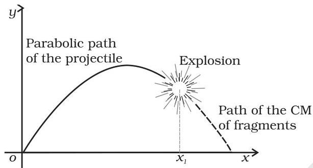Fig. 6.12 The centre of mass of the fragments of the projectile continues along the same parabolic path which it would have followed if there were no explosion.

Figure 6.12 serves as an exemplary demonstration of Equation (6.11). Consider a projectile traversing a standard parabolic path that subsequently detonates into multiple fragments mid-flight. The forces instigating this explosion are inherently internal to the system; consequently, they exert no influence on the motion of the center of mass. The cumulative external force, specifically the gravitational force acting on the object, remains invariant both prior to and following the explosive event. Therefore, the center of mass, solely governed by this external force, persists along the identical parabolic trajectory it would have pursued had the explosion not occurred.

6.4 LINEAR MOMENTUM OF A SYSTEM OF PARTICLES

It is pertinent to recall that the linear momentum of an individual particle is defined by the expression:

$ \mathbf {p} = m \mathbf {v} \tag {6.12} $

Furthermore, Newton's second law, when expressed symbolically for a single particle, states:

$ \mathbf {F} = \frac {\mathrm {d} \mathbf {p}}{\mathrm {d} t} \tag {6.13} $

where $\mathbf{F}$ signifies the force acting upon the particle. Now, consider a system comprising $n$ discrete particles, each possessing a mass $m_{i}$ and a velocity $\mathbf{v}{i}$, for $i = 1, 2, \ldots, n$. These particles are subject to both internal interactions and external forces. Consequently, the linear momentum for the first particle is $m{1} \mathbf{v}{1}$, for the second particle is $m{2} \mathbf{v}_{2}$, and so forth.

For such a system of $n$ particles, the aggregate linear momentum of the system is formally established as the vector summation of the momenta of its constituent individual particles:

$ \begin{array}{l} \mathbf {P} = \mathbf {p} _ {1} + \mathbf {p} _ {2} + \dots + \mathbf {p} _ {n} \ = m _ {1} \mathbf {v} _ {1} + m _ {2} \mathbf {v} _ {2} + \dots + m _ {n} \mathbf {v} _ {n} \tag {6.14} \ \end{array} $

A comparison with Equation (6.8) reveals that:

$ \mathbf {P} = M \mathbf {V} \tag {6.15} $

Hence, the collective momentum of a particle system is equivalent to the product of its total mass and the velocity of its center of mass. Upon differentiation of Equation (6.15) with respect to time, we obtain:

$ \frac {\mathrm {d} \mathbf {P}}{\mathrm {d} t} = M \frac {\mathrm {d} \mathbf {V}}{\mathrm {d} t} = M \mathbf {A} \tag {6.16} $

By comparing Equation (6.16) with Equation (6.11), it follows that:

$ \frac {\mathrm {d} \mathbf {P}}{\mathrm {d} t} = \mathbf {F} _ {\text {e x t}} \tag {6.17} $

This expression represents the extension of Newton's second law of motion to a system encompassing multiple particles.

Consider a scenario where the resultant external force exerted upon a system of particles is null. In such a circumstance, Equation (6.17) implies:

$ \frac {\mathrm {d} \mathbf {P}}{\mathrm {d} t} = 0 \quad \text {or} \quad \mathbf {P} = \text {Constant} \tag {6.18a} $

Consequently, if the aggregate external force acting on a particle system is absent, the system's total linear momentum is conserved. This principle is formally known as the law of conservation of total linear momentum for a system of particles. In light of Equation (6.15), this further indicates that an absence of net external force on the system results in a constant velocity for its center of mass. (It is presupposed throughout the current chapter's discourse on particle systems that the total mass of the system remains invariant.)

It is important to recognize that while internal forces—those exchanged between the particles themselves—can induce intricate trajectories for individual particles

, should the net external force on the system be zero, the center of mass will nonetheless exhibit motion at a constant velocity, thereby traversing a uniform, rectilinear path analogous to that of a free particle.

Vector Equation (6.18a) can be decomposed into three corresponding scalar equations:

$ P_{x} = c_{1}, P_{y} = c_{2} \text{ and } P_{z} = c_{3} \tag{6.18b} $

The quantities $P_{x}, P_{y}$, and $P_{z}$ represent the components of the total linear momentum vector $\mathbf{P}$ along the $x-, y-$, and $z$-axes, respectively, while $c_{1}, c_{2}$, and $c_{3}$ are constants.

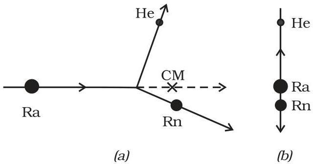Fig. 6.13 (a) A heavy nucleus radium (Ra) splits into a lighter nucleus radon (Rn) and an alpha particle (nucleus of helium atom). The CM of the system is in uniform motion. (b) The same splitting of the heavy nucleus radium (Ra) with the centre of mass at rest. The two product particles fly back to back.

To illustrate this principle, we can examine the radioactive disintegration of an unstable, moving particle, specifically a radium nucleus. Such a nucleus undergoes decay, yielding a radon nucleus and an alpha particle. Since the forces driving this decay originate from within the system, and external forces acting upon it are inconsequential, the aggregate linear momentum of the system remains conserved both prior to and subsequent to the disintegration. The resulting decay products—the radon nucleus and the alpha particle—propagate in divergent trajectories, yet their collective center of mass continues to traverse the identical trajectory initially followed by the decaying radium nucleus [Fig. 6.13(a)].

When the decay event is viewed from a reference frame where the center of mass is stationary, the kinematics of the participating particles appear notably simplified; the resultant particles

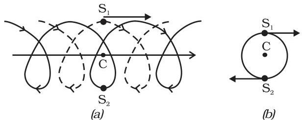Fig. 6.14 (a) Trajectories of two stars, $S_{z}$ (dotted line) and $S_{y}$ (solid line) forming a binary system with their centre of mass $C$ in uniform motion. (b) The same binary system, with the centre of mass $C$ at rest.

recede from each other in opposite directions, with their center of mass maintaining its stationary state, as illustrated in Fig. 6.13(b).

For numerous problems involving particle systems, such as the aforementioned radioactive decay scenario, employing the center of mass frame often proves more advantageous than utilizing the laboratory reference frame.

The phenomenon of binary (or double) star systems is frequently observed in astronomical contexts. Absent any external forces, the center of mass of such a stellar pair exhibits motion characteristic of a free particle, as depicted in Fig. 6.14(a). The paths traced by two stars of equivalent mass are also illustrated, appearing intricate. However, upon transitioning to the center of mass frame, it becomes evident that the two stars execute circular motion around their stationary center of mass. It is important to note that the stars must occupy positions diametrically opposed to one another [Fig. 6.14(b)]. Consequently, within our observational frame, the stellar trajectories represent a superposition of (i) the uniform rectilinear motion of the center of mass and (ii) the orbital circular paths of the stars around this center of mass.

As demonstrated by these two examples, decomposing the motion of a system's constituent parts into the motion of the center of mass and the motion relative to the center of mass constitutes a highly effective technique for comprehending the system's overall dynamics.

6.5 VECTOR PRODUCT OF TWO VECTORS

Our previous discussions have established the concept of vectors and their applications in physics. Chapter 5, focusing on Work, Energy, and Power, introduced the scalar product of two vectors. Work, a crucial physical quantity, is specifically defined as the scalar product of two vector entities: force and displacement.

This section will introduce a distinct type of product involving two vectors, which itself yields a vector. Key quantities central to the analysis of rotational motion, such as the moment of a force and angular momentum, are characterized as vector products.

Definition of Vector Product

The vector product of two given vectors, $\mathbf{a}$ and $\mathbf{b}$, results in a third vector, $\mathbf{c}$, defined by the following characteristics:

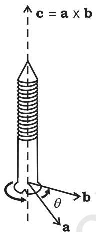
(i) The scalar magnitude of $\mathbf{c}$, denoted as $c$, is given by $ab\sin \theta$, where $a$ and $b$ represent the magnitudes of vectors $\mathbf{a}$ and $\mathbf{b}$ respectively, and $\theta$ is the angle subtended between them. (ii) The resultant vector $\mathbf{c}$ lies perpendicular to the plane defined by vectors $\mathbf{a}$ and $\mathbf{b}$. (iii) To ascertain the direction of $\mathbf{c}$, one can employ the right-handed screw rule: if a right-handed screw, positioned with its head in the plane of $\mathbf{a}$ and $\mathbf{b}$ and its axis normal to this plane, is rotated such that its head turns from the direction of $\mathbf{a}$ towards $\mathbf{b}$, then the screw's tip will advance in the direction of $\mathbf{c}$. This principle is depicted in Fig. 6.15a.

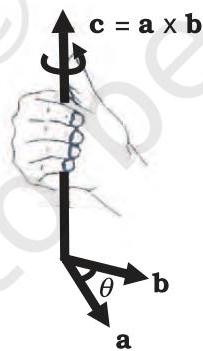
An alternative method for determining direction involves the right-hand rule: if the fingers of the right hand are curled in the direction of rotation from vector $\mathbf{a}$ to vector $\mathbf{b}$ around an axis perpendicular to their plane, then the extended thumb indicates the direction of vector $\mathbf{c}$, as illustrated in Fig. 6.15b.

(a) Fig. 6.15 (a) Rule of the right handed screw for defining the direction of the vector product of two vectors. (b) Rule of the right hand for defining the direction of the vector product.

(b)

A more simplified interpretation of the right-hand rule is as follows: Extend the palm of your right hand and curl your fingers from vector $\mathbf{a}$ towards vector $\mathbf{b}$. Your extended thumb will then indicate the direction of $\mathbf{c}$.

It is important to note that any two vectors, $\mathbf{a}$ and $\mathbf{b}$, define two distinct angles between them. As depicted in Fig. 6.15 (a) or (b), these are $\theta$ (the illustrated angle) and $(360^{\circ} - \theta)$. When applying either of the directional rules previously described, the rotation must always be considered through the acute angle (i.e., less than $180^{\circ}$) between $\mathbf{a}$ and $\mathbf{b}$. In this context, $\theta$ represents that smaller angle.

The vector product is frequently termed the "cross product" due to the symbol $(\mathbf{x})$ employed in its notation.

• It should be recalled that, as previously discussed, the scalar product of two vectors exhibits commutativity; that is, $\mathbf{a}.\mathbf{b} = \mathbf{b}.\mathbf{a}$.

Conversely, the vector product does not possess the property of commutativity, meaning $\mathbf{a} \times \mathbf{b} \neq \mathbf{b} \times \mathbf{a}$.

While the magnitudes of both $\mathbf{a} \times \mathbf{b}$ and $\mathbf{b} \times \mathbf{a}$ are identical ($ab\sin \theta$) and both resultant vectors are orthogonal to the plane containing $\mathbf{a}$ and $\mathbf{b}$, their directions differ. Specifically, the right-handed screw rotation for $\mathbf{a} \times \mathbf{b}$ proceeds from $\mathbf{a}$ to $\mathbf{b}$, whereas for $\mathbf{b} \times \mathbf{a}$ it proceeds from $\mathbf{b}$ to $\mathbf{a}$. Consequently, these two vector products point in diametrically opposite directions. We thus observe:

$ \mathbf{a} \times \mathbf{b} = -\mathbf{b} \times \mathbf{a} $

• An additional noteworthy characteristic of the vector product pertains to its behavior under reflection. When subjected to a reflection (conceptualized as generating a plane mirror image), the coordinate axes transform as $x \rightarrow -x, y \rightarrow -y$, and $z \rightarrow -z$. Consequently, all components of a vector reverse their signs, leading to transformations $a \rightarrow -a$ and $b \rightarrow -b$. The question then arises: what is the effect of reflection on the vector product $\mathbf{a} \times \mathbf{b}$?

$ \mathbf{a} \times \mathbf{b} \rightarrow (-\mathbf{a}) \times (-\mathbf{b}) = \mathbf{a} \times \mathbf{b} $

Thus, the vector product $\mathbf{a} \times \mathbf{b}$ exhibits invariance in sign when undergoing reflection.

• Both the scalar product (dot product) and the vector product (cross product) demonstrate distributivity over vector addition. Specifically, this means:

$ \mathbf{a}.\left(\mathbf{b} + \mathbf{c}\right) = \mathbf{a}.\mathbf{b} + \mathbf{a}.\mathbf{c} $

$ \mathbf{a} \times (\mathbf{b} + \mathbf{c}) = \mathbf{a} \times \mathbf{b} + \mathbf{a} \times \mathbf{c} $

• To express the vector $\mathbf{c} = \mathbf{a} \times \mathbf{b}$ in its component form, it is first necessary to establish certain fundamental cross products:

(i) $\mathbf{a} \times \mathbf{a} = \mathbf{0}$ ($\mathbf{0}$ denotes a null vector, which is a vector possessing zero magnitude)

This conclusion is derived from the fact that the magnitude of $\mathbf{a} \times \mathbf{a}$ is given by $a^2 \sin 0^\circ = 0$.

SYSTEMS OF PARTICLES AND ROTATIONAL MOTION

From this principle, the following specific results are deduced:

(i) $\hat{\mathbf{i}}\times \hat{\mathbf{i}} = \mathbf{0},\hat{\mathbf{j}}\times \hat{\mathbf{j}} = \mathbf{0},\hat{\mathbf{k}}\times \hat{\mathbf{k}} = \mathbf{0}$ (ii) $\hat{\mathbf{i}}\times \hat{\mathbf{j}} = \hat{\mathbf{k}}$

It is important to recognize that the magnitude of $\hat{\mathbf{i}}\times \hat{\mathbf{j}}$ evaluates to $\sin 90^{\circ}$, which is 1, because both $\hat{\mathbf{i}}$ and $\hat{\mathbf{j}}$ are unit vectors and are separated by an angle of $90^{\circ}$. Consequently, $\hat{\mathbf{i}}\times \hat{\mathbf{j}}$ itself constitutes a unit vector. According to the right-hand screw rule, the unit vector that is perpendicular to the plane defined by $\hat{\mathbf{i}}$ and $\hat{\mathbf{j}}$ is $\hat{\mathbf{k}}$. This explains the aforementioned result. One can similarly verify:

$ \hat {\mathbf {j}} \times \hat {\mathbf {k}} = \hat {\mathbf {i}} \quad \text {and} \quad \hat {\mathbf {k}} \times \hat {\mathbf {i}} = \hat {\mathbf {j}} $

Applying the anti-commutative property of the cross product, it logically follows:

$ \hat {\mathbf {j}} \times \hat {\mathbf {i}} = - \hat {\mathbf {k}}, \quad \hat {\mathbf {k}} \times \hat {\mathbf {j}} = - \hat {\mathbf {i}}, \quad \hat {\mathbf {i}} \times \hat {\mathbf {k}} = - \hat {\mathbf {j}} $

Observe that if the unit vectors $\hat{\mathbf{i}},\hat{\mathbf{j}},\hat{\mathbf{k}}$ appear in a cyclic sequence within the vector product relation, the resulting vector product is positive. Conversely, if $\hat{\mathbf{i}},\hat{\mathbf{j}},\hat{\mathbf{k}}$ do not maintain a cyclic order, the vector product will be negative.

Now,

$ \begin{array}{l} \mathbf {a} \times \mathbf {b} = \left(a _ {x} \hat {\mathbf {i}} + a _ {y} \hat {\mathbf {j}} + a _ {z} \hat {\mathbf {k}}\right) \times \left(b _ {x} \hat {\mathbf {i}} + b _ {y} \hat {\mathbf {j}} + b _ {z} \hat {\mathbf {k}}\right) \ = a _ {x} b _ {y} \hat {\mathbf {k}} - a _ {x} b _ {z} \hat {\mathbf {j}} - a _ {y} b _ {x} \hat {\mathbf {k}} + a _ {y} b _ {z} \hat {\mathbf {i}} + a _ {z} b _ {x} \hat {\mathbf {j}} - a _ {z} b _ {y} \hat {\mathbf {i}} \ = \left(a _ {y} b _ {z} - a _ {z} b _ {y}\right) \hat {\mathbf {i}} + \left(a _ {z} b _ {x} - a _ {x} b _ {z}\right) \hat {\mathbf {j}} + \left(a _ {x} b _ {y} - a _ {y} b _ {x}\right) \hat {\mathbf {k}} \ \end{array} $

The aforementioned relationship was derived using fundamental cross product operations. The vector product $\mathbf{a} \times \mathbf{b}$ can be concisely represented in a determinant structure, which aids memorization.

$ \mathbf {a} \times \mathbf {b} = \left| \begin{array}{c c c} \hat {\mathbf {i}} & \hat {\mathbf {j}} & \hat {\mathbf {k}} \ a _ {x} & a _ {y} & a _ {z} \ b _ {x} & b _ {y} & b _ {z} \end{array} \right| $

Example 6.4 Find the scalar and vector products of two vectors. $\mathbf{a} = (3\hat{\mathbf{i}} - 4\hat{\mathbf{j}} + 5\hat{\mathbf{k}})$ and $\mathbf{b} = (-2\hat{\mathbf{i}} + \hat{\mathbf{j}} + 3\hat{\mathbf{k}})$

Answer

$ \begin{array}{l} \mathbf {a} \cdot \mathbf {b} = (3 \hat {\mathbf {i}} - 4 \hat {\mathbf {j}} + 5 \hat {\mathbf {k}}) \cdot (- 2 \hat {\mathbf {i}} + \hat {\mathbf {j}} - 3 \hat {\mathbf {k}}) \ = - 6 - 4 - 1 5 \ = - 2 5 \ \end{array} $

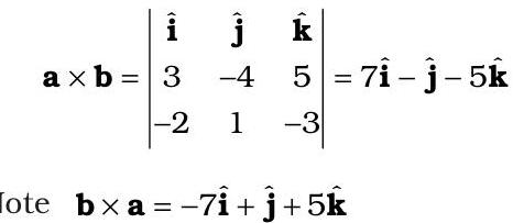
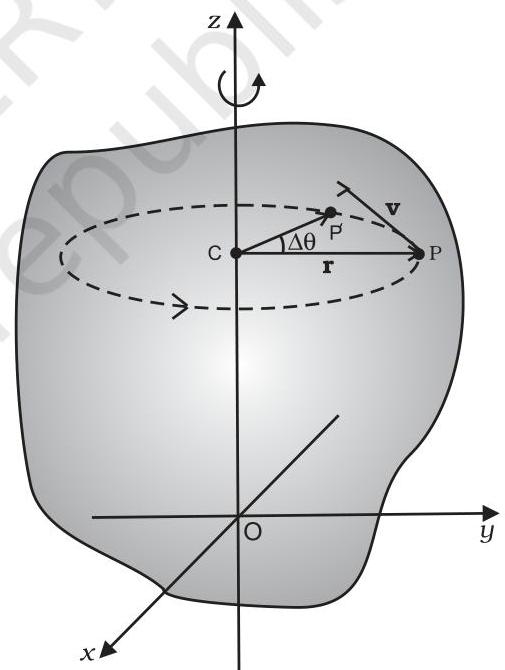Fig. 6.16 Rotation about a fixed axis. (A particle $(P)$ of the rigid body rotating about the fixed $(z-)$ axis moves in a circle with centre $(C)$ on the axis.)

The trajectory of this particle is a circular path situated within a plane orthogonal to the axis, with its center coinciding with the axis. Figure 6.16, a modified depiction of Fig. 6.4, illustrates a representative particle (at point P) belonging to a rigid body undergoing rotation around a stationary axis (designated as the $z$-axis). This particle

traces out a circular trajectory, centered at C on the axis. The radius of this circle, denoted by $r$, represents the perpendicular distance from point P to the axis. The linear velocity vector $\mathbf{v}$ of the particle at P is also depicted, oriented tangentially to the circle at that point.

Consider $\mathrm{P}'$ as the particle's location after a time duration $\Delta t$ (refer to Fig. 6.16). The angular separation $\mathrm{PCP}'$ quantifies the angular displacement, $\Delta \theta$, experienced by the particle during this interval $\Delta t$. The average angular velocity of the particle over the period $\Delta t$ is defined as $\Delta \theta / \Delta t$. As $\Delta t$ approaches zero (i.e., diminishing progressively), the quotient $\Delta \theta / \Delta t$ converges to a limiting value, which represents the instantaneous angular velocity, $\mathrm{d}\theta / \mathrm{d}t$, of the particle at position P. This instantaneous angular velocity is symbolized by $\omega$ (the Greek letter omega). From our previous examination of circular motion, we recall that the scalar magnitude of the linear velocity, $\nu$, for a particle executing circular motion, maintains a straightforward relationship with its angular velocity, $\omega$, expressed as $\upsilon = \omega r$, where $r$ signifies the circle's radius.

It is noteworthy that at any specific moment, the relationship $v = \omega r$ is valid for every particle within the rigid body. Consequently, for any particle situated at a perpendicular distance $r_i$ from the fixed axis, its linear velocity $v_i$ at a particular instant is expressed as:

$ v _ {i} = \omega r _ {i} \tag {6.19} $

The index $i$ runs from 1 to $n$, where $n$ is the total number of particles of the body.

Particles situated on the rotational axis possess a radial distance $r = 0$, which consequently leads to a linear velocity $v = \omega r = 0$. Therefore, these particles remain motionless, confirming the immobility of the axis itself.

It is important to recognize that a uniform angular velocity, denoted as $\omega$, is attributed to every particle within the system. Consequently, $\omega$ is designated as the angular velocity characteristic of the entire rigid body.

Pure translational motion of a body has been defined by the condition where all its constituent parts possess an identical linear velocity at any given moment. Analogously, pure rotational motion can be characterized by the state where all components of the body exhibit the same angular velocity at any instantaneous point in time. This description of a rigid body's rotation around a fixed axis is, in essence, a restatement of the principle articulated in Section 6.1: every particle within the body executes circular motion within a plane orthogonal to the axis, with the center of this circle located directly on the axis.

Up to this point in our analysis, angular velocity has been presented as a scalar quantity. However, it is fundamentally a vector. While a formal justification for this assertion will not be provided here, we will proceed by accepting it as a given. In the context of rotation around a fixed axis, the angular velocity vector is oriented precisely along the axis of rotation, and its direction corresponds to the advancement of a right-handed screw if its head were rotated in concordance with the body's motion. (Refer to Fig. 6.17a).

The scalar magnitude of this vector is given by $\omega = \mathrm{d}\theta / \mathrm{d}t$, as previously mentioned.

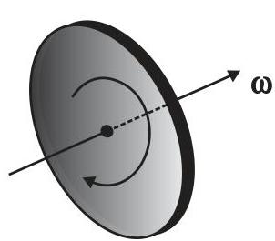Fig. 6.17 (a) If the head of a right handed screw rotates with the body, the screw advances in the direction of the angular velocity $\omega$. If the sense (clockwise or anticlockwise) of rotation of the body changes, so does the direction of $\omega$.

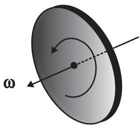
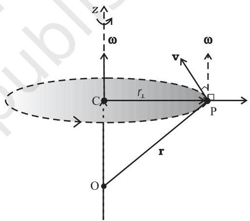Fig. 6.17 (b) The angular velocity vector $\omega$ is directed along the fixed axis as shown. The linear velocity of the particle at $P$ is $\mathbf{v} = \boldsymbol{\omega} \times \mathbf{r}$. It is perpendicular to both $\boldsymbol{\omega}$ and $\mathbf{r}$ and is directed along the tangent to the circle described by the particle.

Our attention will now turn to the physical interpretation of the vector product $\omega \times \mathbf{r}$. Consult Fig. 6.17(b), which is an excerpt from Fig. 6.16, presented to illustrate the trajectory of particle P. This diagram depicts the vector $\omega$ aligned with the stationary $(z-)$ axis, alongside the position vector $\mathbf{r} = \mathbf{OP}$ representing particle P within the rigid body relative to the origin O. It is important to note that the chosen origin coincides with the axis of rotation.

SYSTEMS OF PARTICLES AND ROTATIONAL MOTION

Now $\omega \times \mathbf{r} = \omega \times \mathbf{OP} = \omega \times (\mathbf{OC} + \mathbf{CP})$

However, $\omega \times \mathbf{OC} = 0$ because $\omega$ is collinear with OC.

Hence $\omega \times \mathbf{r} = \omega \times \mathbf{CP}$

The vector $\boldsymbol{\omega} \times \mathbf{CP}$ is orthogonal to both $\boldsymbol{\omega}$ (which is aligned with the $z$-axis) and $\mathbf{CP}$, the radius vector delineating the particle's circular path at P. Consequently, its orientation is along the tangent to the circle at P. Furthermore, because $\boldsymbol{\omega}$ and $\mathbf{CP}$ are mutually perpendicular, the magnitude of $\boldsymbol{\omega} \times \mathbf{CP}$ is simply $\omega (\text{CP})$. For clarity, $\mathbf{CP}$ will henceforth be designated as $\mathbf{r}_{\perp}$, distinguishing it from the general position vector $\mathbf{r}$ used previously.

Therefore, the vector $\boldsymbol{\omega} \times \mathbf{r}$ possesses a magnitude of $\omega r_{\perp}$ and is directed along the tangent to the circular trajectory traced by the particle at P. The linear velocity vector $\mathbf{v}$ at P exhibits this identical magnitude and direction. Hence, we establish the relationship:

$ \mathbf {v} = \boldsymbol {\omega} \times \mathbf {r} \tag {6.20} $

Indeed, this relationship, expressed by Eq. (6.20), extends its validity to the rotation of a rigid body with a single fixed point, exemplifying situations like the motion of a spinning top [Fig. 6.6(a)]. In such contexts, $\mathbf{r}$ signifies the position vector of the particle relative to the fixed point, which is conventionally designated as the origin.

It is pertinent to observe that in the case of rotation around a fixed axis, the directional orientation of the vector $\boldsymbol{\omega}$ remains invariant over time. However, its scalar magnitude is subject to instantaneous fluctuations. Conversely, for more generalized rotational kinematics, both the magnitude and the directional orientation of $\boldsymbol{\omega}$ can undergo instantaneous variations.

6.6.1 Angular acceleration

It is observable that our exploration of rotational dynamics proceeds in parallel with the established framework of translational motion. Just as linear displacement (s) and linear velocity (v) serve as key kinematic parameters in translational contexts, their rotational counterparts are angular displacement (θ) and angular velocity (ω). Consequently, it is a logical progression to introduce angular acceleration within rotational mechanics, mirroring the definition of linear acceleration as the instantaneous rate of change of velocity in translational systems. Specifically, angular acceleration, denoted by $\alpha$, is formally defined as the temporal derivative of angular velocity. Hence,

$ \alpha = \frac {\mathrm {d} \omega}{\mathrm {d} t} \tag {6.21} $

Should the rotational axis remain stationary, both the orientation of $\omega$ and, by extension, that of $\alpha$ become invariant. Under such conditions, the vector formulation simplifies, allowing its representation as a scalar equation:

$ \alpha = \frac {\mathrm {d} \omega}{\mathrm {d} t} \tag {6.22} $

6.7 TORQUE AND ANGULAR MOMENTUM

This forthcoming segment will introduce two fundamental physical quantities, torque and angular momentum, both characterized as the vector cross products of distinct vectors. As will become evident, these concepts hold particular importance in analyzing the motion of particle aggregates, especially rigid bodies.

6.7.1 Moment of force (Torque)

The movement of a rigid body is generally understood as a composite of rotational and translational components. Should a body be constrained at a specific point or along a particular line, its motion becomes exclusively rotational. It is established that a force is requisite for altering a body's translational state, thereby inducing linear acceleration. This prompts the inquiry: what serves as the rotational counterpart to force? To address this in a tangible context, consider the act of opening or closing a door. A door functions as a rigid body, capable of rotation around a fixed vertical axis defined by its hinges. What mechanism instigates this rotation? Evidently, rotation does not occur without the application of a force. However, not all forces achieve this outcome. A force exerted along the hinge line will fail to generate any rotation whatsoever, whereas a force of equivalent magnitude, applied perpendicularly to the door's outer edge, proves maximally effective in inducing rotation. Thus, in rotational dynamics, the efficacy is not solely determined by the force itself, but critically by its point and manner of application.

In the realm of rotational motion, the equivalent of force in linear motion is termed the moment of force, also known as torque or couple. (These terms, moment of force and torque, will be employed synonymously throughout this discussion.) Our initial focus will be on defining the moment of force specifically for an isolated particle. Subsequently, this concept will be expanded to encompass systems of particles, including rigid bodies. Furthermore, we will establish its connection to alterations in rotational motion, specifically the angular acceleration of a rigid body.

Reprint 2025-26

PHYSICS

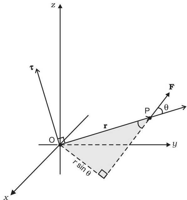Fig. 6.18 $\tau = \mathbf{r} \times \mathbf{F}$ , $\tau$ is perpendicular to the plane containing $\mathbf{r}$ and $\mathbf{F}$ , and its direction is given by the right handed screw rule.

When a force is exerted upon an individual particle situated at point $\mathbf{P}$, with its position relative to the origin $\mathbf{O}$ denoted by the position vector $\mathbf{r}$ (as depicted in Fig. 6.18), the moment of this force, relative to the origin $\mathbf{O}$, is formally defined as the vector product:

$ \tau = \mathbf {r} \times \mathbf {F} \tag {6.23} $

The moment of force (or torque) constitutes a vector quantity. The Greek letter tau is represented by the symbol $\tau$. The scalar magnitude of $\tau$ is given by:

$ \tau = r F \sin \theta \tag {6.24a} $

Here, $r$ denotes the magnitude of the position vector $\mathbf{r}$, which corresponds to the length OP; $F$ signifies the magnitude of the force $\mathbf{F}$; and $\theta$ represents the angle subtended between $\mathbf{r}$ and $\mathbf{F}$, as illustrated.

The dimensional representation of the moment of force is $\mathrm